

Quantum Mechanics by Konstantin K. Likharev - HTML preview
Download the book in PDF, ePub, Kindle for a complete version.
dq / dt
F /
Fa
so their frequency may be expressed by a very simple formula
Bloch
2
Fa
oscillations:
,
(2.244)
B
frequency
t
B
and hence is independent of any peculiarities of the energy band/gap structure.
The direct-space motion of the wave packet’s center x 0( t) during the Bloch oscillation process may be analyzed by integrating the first of Eqs. (235) over some time interval t, and using Eq. (237): 75 This phenomenon may be also discussed from the point of view of the reduced zone picture, but then it requires the introduction of instant jumps between the Brillouin zone boundary points (see the dashed red line in Fig. 33) that correspond to physically equivalent states of the particle. Evidently, for the description of this particular phenomenon, this language is more artificial.
Chapter 2
Page 59 of 76
QM: Quantum Mechanics
t
t
d( q )
t
d( q )
t t
0
0
x
( t) v dt
dt
d
q .
(2.245)
0
gr
0
dq
dq / dt
F
F
0
0
0
0
0
t0
If the interval t is equal to the Bloch oscillation period t B (243), the initial and final values of E( q 0) =
( q 0) are equal, giving x 0 = 0: in the end of the period, the wave packet returns to its initial position in space. However, if we carry out this integration only from the smallest to the largest values of ( q 0), i.e.
the adjacent points where the group velocity vanishes, we get the following Bloch oscillation swing: Bloch
E
x
.
(2.246) oscillations:
max
max
min
1
F
F
spatial
swing
This simple result may be interpreted using an alternative energy diagram (Fig. 33b), which results from the following arguments. The additional force F may be described not only via the 2nd Newton law’s version (237), but, alternatively, by its contribution – Fx to the Gibbs potential energy76
U ( x) U ( x) Fx
(2.247)
The exact solution of the Schrödinger equation (61) with such a potential may be hard to find directly, but if the force F is sufficiently weak, as we are assuming throughout this discussion, the second term in Eq. (247) may be considered as a constant on the scale of a << x max. In this case, our quantum-mechanical treatment of the periodic potential U( x) is still virtually correct, but with an energy shift depending on the “global” position x 0 of the packet’s center. In this approximation, the total energy of the wave packet is
E E( q ) Fx .
(2.248)
0
0
In a plot of such energy as a function of x 0 (Fig. 33b), the energy dependence on q 0 is hidden, but as was discussed above, it is rather uneventful and may be well characterized by the position of bandgap edges on the energy axis.77 In this representation, the Bloch oscillations keep the full energy E of the particle constant, i.e. follow a horizontal line in Fig. 33b, limited by the classical turning points corresponding to the bottom and the top of the allowed energy band. The distance x max between these points is evidently given by Eq. (246).
Besides this alternative look at the Bloch oscillation swing, the total energy diagram shown in Fig. 33b enables one more remarkable result. Let a wave packet be so narrow in the momentum space that x ~ 1/ q >> x max; then it may be well represented by a definite energy, i.e. by a horizontal line in Fig. 33b. But Eq. (247) is exactly invariant with respect to the following simultaneous translation of the coordinate and the energy:
x x a, E E Fa .
(2.249)
76 Physically, this is just the relevant part of the potential energy of the total system comprised of our particle (in the periodic potential) and the source of the force F – see, e.g., CM Sec. 1.4.
77 In semiconductor physics and engineering, such spatial band-edge diagrams are virtually unavoidable components of almost every discussion/publication. In this series, a few more examples of such diagrams may be found in SM Sec. 6.4.
Chapter 2
Page 60 of 76
QM: Quantum Mechanics
This means that it is satisfied by an infinite set of similar solutions, each corresponding to one of the horizontal red lines shown in Fig. 33b. This is the famous Wannier-Stark ladder,78 with the step height Wannier-Stark
E
Fa .
(2.250)
WS
ladder
The importance of this alternative representation of the Bloch oscillations is due to the following fact. In most experimental realizations, the power of electromagnetic radiation with frequency (244), which may be extracted from the oscillations of a charged particle, is very low, so their direct detection represents a hard problem.79 However, let us apply to a Bloch oscillator an additional ac field at frequency B. As these frequencies are brought close together, the external signal should synchronize (“phase-lock”) the Bloch oscillations,80 resulting in certain changes of time-independent observables – for example, a resonant change of absorption of the external radiation. Now let us notice that the combination of Eqs. (244) and (250) yield the following simple relation:
E
.
(2.251)
WS
B
This means that the phase-locking at B allows for an alternative (but equivalent) interpretation – as the result of ac-field-induced quantum transitions81 between the steps of the Wannier-Stark ladder.
(Again, such occasions when two very different languages may be used for alternative interpretations of the same effect is one of the most beautiful features of physics.)
This phase-locking effect has been used for the first experimental confirmations of the Bloch oscillation theory.82 For this purpose, the natural periodic structures, solid-state crystals, are inconvenient due to their very small period a ~ 10-10 m. Indeed, according to Eq. (244), such structures require very high forces F (and hence very high electric fields E = F/ e) to bring B to an experimentally convenient range. This problem has been overcome using artificial periodic structures ( superlattices) of certain semiconductor compounds, such as Ga1- x Al x As with various degrees x of the gallium-to-aluminum atom replacement, whose layers may be grown over each other epitaxially, i.e., with very few crystal structure violations. Such superlattices, with periods a ~ 10 nm, have enabled a clear observation of the resonance at B, and hence a measurement of the Bloch oscillation frequency, in particular its proportionality to the applied dc electric field, predicted by Eq. (244).
Very soon after this discovery, the Bloch oscillations were observed83 in small Josephson junctions, where they result from the quantum dynamics of the Josephson phase difference in a 2-
periodic potential profile, created by the junction. A straightforward translation of Eq. (244) to this case (left for the reader’s exercise) shows that the frequency of such Bloch oscillations is 78 This effect was first discussed in detail by G. Wannier in his 1959 monograph on solid-state physics, while the name of J. Stark is traditionally associated with virtually any electric field effect on atomic systems after he had discovered the first of such effects in 1913 – see its discussion in Sec. 6.2 below.
79 In systems with many independent particles (such as electrons in semiconductors), the detection problem is exacerbated by the phase incoherence of the Bloch oscillations performed by each particle. This drawback is absent in atomic Bose-Einstein condensates whose Bloch oscillations (in a periodic potential created by standing optical waves) were eventually observed by M. Ben Dahan et al., Phys. Rev. Lett. 76, 4508 (1996).
80 A simple analysis of the phase locking of a classical oscillator may be found, e.g., in CM Sec. 5.4. (See also the brief discussion of the phase locking of the Josephson oscillations at the end of Sec. 1.6 of this course.) 81 A quantitative theory of such transitions will be discussed in Sec. 6.6 and then in Chapter 7.
82 E. Mendez et al., Phys. Lev. Lett. 60, 2426 (1988).
83 D. Haviland et al. , Z. Phys. B 85, 339 (1991).
Chapter 2
Page 61 of 76
QM: Quantum Mechanics
I
I
,
i.e. f
B
,
(2.252)
B
2 e
B
2
2 e
where I is the dc current passed through the junction – the effect not to be confused with the “classical”
Josephson oscillations with frequency (1.75). It is curious that Eq. (252) may be legitimately interpreted as a result of a periodic transfer, through the Josephson junction, of discrete Cooper pairs (with electric charge –2 e each), between two coherent Bose-Einstein condensates in the superconducting electrodes of the junction.84
So far, our discussion of the Bloch oscillations was based on the premise that the wave packet of the particle stays within one (say, the lowest) energy band. However, just one look at Fig. 28 shows that this assumption becomes unrealistic if the energy gap separating this band from the next one becomes very small, 1 0. Indeed, in the weak-potential approximation, which is adequate in this limit, U 1
0, the two dispersion curve branches (216) cross without any interaction, so if our particle (meaning its the wave packet) is driven to approach that point, it should continue to move up in energy – see the dashed blue arrow in Fig. 33a. Similarly, in the real-space representation shown in Fig. 33b, it is intuitively clear that at 1 0, the particle residing at one of the steps of the Wannier-Stark ladder should be able to somehow overcome the vanishing spatial gap x 0 = 1/ F and to “leak” into the next band – see the horizontal dashed blue arrow on that panel.
This process, called the Landau-Zener (or “interband”, or “band-to-band”) tunneling,85 is indeed possible. To analyze it, let us first take F = 0, and consider what happens if a quantum particle, described by an x-long (and hence E-narrow) wave packet, is incident from free space upon a periodic structure of a large but finite length l = Na >> a – see, e.g., Fig. 22. If the packet’s energy E is within one of the energy bands, it may evidently propagate through the structure (though may be partly reflected from its ends). The corresponding quasimomentum may be found by solving the dispersion relation for q; for example, in the weak-potential limit, Eq. (224) (which is valid near the gap) yields 1
~
~
~
1/ 2
2
2
2
~
q q q, with q
(2.253)
m
E Un , for
2
U
E ,
n
~
where
( n)
E E E and = 2 aE( n)/ n – see the second of Eqs. (225).
Now, if the energy E is inside one of the energy gaps n, the wave packet’s propagation in an infinite periodic lattice is impossible, so it is completely reflected from it. However, our analysis of the potential step problem in Sec. 3 implies that the packet’s wavefunction should still have an exponential tail protruding into the structure and decaying on some length – see Eq. (58) and Fig. 2.4. Indeed, a straightforward review of the calculations leading to Eq. (253) shows that it remains valid for energies within the gap as well, if the quasimomentum is understood as a purely imaginary number: 1/ 2
1
~
~
~
q i,
where
2
2
U
E
E U
.
(2.254)
n
2
2
,
for
n
84 See, e.g., D. Averin et al., Sov. Phys. – JETP 61, 407 (1985). This effect is qualitatively similar to the transfer of single electrons, with a similar frequency f = I/ e, in tunnel junctions between “normal” (non-superconducting) metals – see, e.g., EM Sec. 2.9 and references therein.
85 It was predicted, apparently independently, by L. Landau, C. Zener, E. Stueckelberg, and E. Majorana in 1932.
Chapter 2
Page 62 of 76
QM: Quantum Mechanics
With this replacement, the Bloch solution (193b) indeed describes an exponential decay of the wavefunction at length ~ 1/.
Returning to the effects of weak force F, in the real-space approach described by Eq. (248) and illustrated in Fig. 33b, we may recast Eq. (254) as
1/
1
( x)
2
~ 2
U
( x
F )
,
(2.255)
n
2
where x~ is the particle’s (i.e. its wave packet center’s) deviation from the midgap point. Thus the gap creates a potential barrier of a finite width x 0 = 2 Un/ F, through which the wave packet may tunnel with a non-zero probability. As we already know, in the WKB approximation (in our case requiring
x 0 >> 1) this probability is just the potential barrier’s transparency T, which may be calculated from Eq. (117):
xc
1
1/ 2
2
2 U
lnT 2 ( x) dx
2
U
~ 2
( x
F
.
(2.256)
n
~
)
x
d
n 2 x 1 2
d
c
1/2
2
( x) 0
x
0
c
where x c x 0/2 = Un / F are the classical turning points. Working out this simple integral (or just noticing that it is a quarter of the unit circle’s area, and hence is equal to /4), we get Landau-Zener
U 2
n
tunneling
T exp
.
(2.257)
probability
F
This famous result may be also obtained in a more complex way, whose advantage is a constructive proof that Eq. (257) is valid for an arbitrary relation between F and Un 2, i.e. arbitrary T, while our simple derivation was limited to the WKB approximation, valid only at T << 1.86 Using Eq.
(225), we may rewrite the product F participating in Eq. (257), as
1 d E E
dq
d E E
l
l
l
l
u
'
0
'
F
,
(2.258)
2
dq
( n)
dt
2
dt
( n)
2
0
E E E
E E E
l
l'
l
l'
where u has the meaning of the “speed” of the energy level crossing in the absence of the gap. Hence, Eq. (257) may be rewritten in the form
U 2
2
n
T exp
,
(2.259)
u
which is more transparent physically. Indeed, the fraction 2 Un / u = n/ u gives the time scale t of the energy’s crossing the gap region, and according to the Fourier transform, its reciprocal, max ~ 1/ t gives the upper cutoff of the frequencies essentially involved in the Bloch oscillation process. Hence Eq.
(259) means that
ln
n
T
.
(2.260)
max
86 In Chapter 6 below, Eq. (257) will be derived using a different method, based on the so-called Golden Rule of quantum mechanics, but also in the weak-potential limit, i.e. for hyperbolic dispersion law (253).
Chapter 2
Page 63 of 76


Essential Graduate Physics
QM: Quantum Mechanics
This formula allows us to interpret the Landau-Zener tunneling as the system’s excitation across the energy gap n by the highest-energy quantum max available from the Bloch oscillation process. This interpretation remains valid even in the opposite, tight-binding limit, in which, according to Eqs. (206) and (237), the Bloch oscillations are purely sinusoidal, so the Landau-Zener tunneling is completely suppressed at B < 1.
Such interband tunneling is an important ingredient of several physical phenomena and even some practical electron devices, for example, the tunneling (or “Esaki”) diodes. This simple device is just a junction of two semiconductor electrodes, one of them so strongly n-doped by electron donors that some electrons form a degenerate Fermi gas at the bottom of the conduction band. 87 Similarly, the counterpart semiconductor electrode is p-doped so strongly that the Fermi level in the valence band is shifted below the band edge – see Fig. 34.
(a)
(b)
(c)
I
n-doped
eV
p-doped
eV
0
/ e
V
Fig. 2.34. The tunneling (“Esaki”) diode: (a) the band-edge diagram of the device at zero bias; (b) the same diagram at a modest positive bias eV ~ /2, and (c) the I-V curve of the device (schematically). Dashed lines on panels (a) and (b) show the Fermi-level positions.
In thermal equilibrium, and in the absence of external voltage bias, the Fermi levels of the two electrodes self-align, leading to the build-up of the contact potential difference / e, with a bit larger than the energy bandgap – see Fig. 34a. This potential difference creates an internal electric field that tilts the energy bands (just as the external field did in Fig. 33b), and leads to the formation of the so-called depletion layer, in which the Fermi level is located within the energy gap and hence there are no charge carriers ready to move. In the usual p-n junctions, this layer is broad and prevents any current at applied voltages V lower than ~/ e. In contrast, in a tunneling diode the depletion layer is so thin (below
~10 nm) that the interband tunneling is possible and provides a substantial Ohmic current at small applied voltages – see Fig. 34c. However, at larger positive biases, with eV ~ /2, the conduction band is aligned with the middle of the energy gap in the p- doped electrode, and electrons cannot tunnel there.
Similarly, there are no electrons in the n-doped semiconductor to tunnel into the available states just above the Fermi level in the p-doped electrode – see Fig. 34b. As a result, at such voltages the current drops significantly, to grow again only when eV exceeds ~, enabling electron motion within each energy band. Thus the junction’s I-V curve has a part with negative differential resistance ( dV/ dI < 0) –
see Fig. 34c. This phenomenon, equivalent in its effect to negative kinematic friction in mechanics, may 87 Here I have to rely on the reader’s background knowledge of basic semiconductor physics; this picture will be discussed in more detail in SM Sec. 6.4.
Chapter 2
Page 64 of 76
QM: Quantum Mechanics
be used for amplification of weak analog signals, for self-excitation of electronic oscillators88 (i.e. an ac signal generation), and for signal swing restoration in digital electronics.
2.9. Harmonic oscillator: Brute force approach
To complete our review of the basic 1D wave mechanics, we have to consider the famous harmonic oscillator, i.e. a 1D particle moving in the quadratic-parabolic potential (111). For it, the stationary Schrödinger equation (53) reads
2
d
2
m 2 x 2
0
E .
(2.261)
2 m dx 2
2
Conceptually, on the background of the fascinating quantum effects discussed in the previous sections, this is not a very interesting system: Eq. (261) is just a standard 1D eigenproblem, resulting in a discrete energy spectrum En, with smooth eigenfunctions n( x) vanishing at x (because the potential energy tends to infinity there).89 However, as we will repeatedly see later in the course, this problem’s solutions have an enormous range of applications, so we have to know their basic properties.
The direct analytical solution of the problem is not very simple (see below), so let us start by trying some indirect approaches to it. First, as was discussed in Sec. 4, the WKB-approximation-based Wilson-Sommerfeld quantization rule (110), applied to this potential, yields the eigenenergy spectrum (114). With the common quantum number convention, this result is
Harmonic
oscillator:
1
energy
E
,
(2.262)
n
n
,
with n
...
2,
1,
0,
0
levels
2
so (in contrast to the 1D rectangular potential well) the ground-state energy corresponds to n = 0.
However, as was discussed in the end of Sec. 4, for the quadratic potential (111) the WKB
approximation’s conditions are strictly satisfied only at En >> 0, so at this point, we can only trust Eq.
(262) for high levels, with n >> 1, rather than for the (most important) ground state.
This is why let me use Eq. (261) to demonstrate another approximate approach, called the variational method, whose simplest form is aimed at finding ground states. The method is based on the following observation. (Here I am presenting its 1D wave mechanics form, though the method is much more general.) Let n be the exact, full, and orthonormal set of stationary wavefunctions of the system under study, and En the set of the corresponding energy levels, satisfying Eq. (1.60): H ˆ E .
(2.263)
n
n
n
Then we may use this set for the unique expansion of an arbitrary trial wavefunction:
,
that
so
*
* *
(2.264)
n
n
,
trial
trial
n
n
n
n
88 See, e.g., CM Sec. 5.4.
89 The stationary state of the harmonic oscillator (which, as will be discussed in Secs. 5.4 and 7.1, may be considered as the state with a definite number of identical bosonic excitations) is sometimes called its Fock state –
after V. A. Fock. (This term is also used in a more general sense, for definite-particle-number states of systems with indistinguishable bosons of any kind – see Sec. 8.3.)
Chapter 2
Page 65 of 76
QM: Quantum Mechanics
where n are some (generally, complex) coefficients. Let us require the trial function to be normalized, using the condition (1.66) of orthonormality of the eigenfunctions n:
*
3
* *
3
*
*
3
*
d x
d x
d x
W
, (2.265)
n
n
n'
n'
n'
n n n'
n'
n
n,n'
1
trial
trial
n
n, n'
n, n'
n, n'
n
where each of the coefficients Wn, defined as
2
*
W
,
0
(2.266)
n
n
n
n
may be interpreted as the probability for the particle, in the trial state, to be found in the n th genuine stationary state. Now let us use Eq. (1.23) for a similar calculation of the expectation value of the system’s Hamiltonian in the trial state:
*
ˆ
3
* * ˆ
3
*
*
3
H
H d x H d x E d x n
n
n'
n'
trial
trial
n'
n
n'
trial
n
n'
n, n'
n, n'
(2.267)
*
E W E
n'
n
n'
n,n'
.
n
n
n, n'
n
Since the exact ground state energy E g is, by definition, the lowest one of the set En, i.e. En E g, Eqs.
(265) and (267) yield the following inequality:
Variational
H
W E E W E .
(2.268)
n
g
g
n
g
method’s
trial
n
n
justification
Thus, the genuine ground state energy of the system is always lower than (or equal to) its energy in any trial state. Hence, if we make several attempts with reasonably selected trial wavefunctions, we may expect the lowest of the results to approximate the genuine ground state energy reasonably well.
Even more conveniently, if we select some reasonable class of trial wavefunctions dependent on a free parameter , then we may use the necessary condition of the minimum of Htrial,
H
trial 0 ,
(2.269)
to find the closest of them to the genuine ground state. Sometimes, even better results may be obtained using trial wavefunctions dependent on several parameters. Note, however, that the variational method does not tell us how exactly the trial function should be selected, or how close its final result is to the genuine ground-state function. In this sense, this method has “uncontrollable accuracy”, and differs from both the WKB approximation and the perturbation methods (to be discussed in Chapter 6), for which we have certain accuracy criteria. Because of this drawback, the variational method is typically used as the last resort – though sometimes (as in the example that follows) it works remarkably well.90
Let us apply this method to the harmonic oscillator. Since the potential (111) is symmetric with respect to point x = 0, and continuous at all points (so, according to Eq. (261), d 2/ dx 2 has to be continuous as well), the most natural selection of the ground-state trial function is the Gaussian function 90 The variational method may be used also to estimate the first excited state (or even a few lowest excited states) of the system, by requiring the new trial function to be orthogonal to the previously calculated eigenfunctions of the lower-energy states. However, the method’s error typically grows with the state number.
Chapter 2
Page 66 of 76
QM: Quantum Mechanics
x C 2
exp x ,
(2.270)
trial
with some real > 0. The normalization coefficient C may be immediately found either from the standard Gaussian integration of trial2, or just from the comparison of this expression with Eq. (16), in which = 1/(2 x)2, i.e. x = 1/21/2, giving C 2 = (2/)1/2. Now the expectation value of the particle’s Hamiltonian,
ˆ 2
2
2
2
2
p
d
m x
ˆ
H
U x
0
,
(2.271)
2 m
2
2
m dx
2
in the trial state, may be calculated as
2
2
2
2
*
d
m x
0
H
dx
trial
trial
2
2
m dx
2
trial
(2.272)
2 1/ 2
2
m
2
2 2
exp 2 2
x
0
2
2
dx
x
exp 2 2
x dx.
m
2
m
0
0
Both involved integrals are of the same well-known Gaussian type,91 giving
2
2
0
H
m
.
(2.273)
trial
2 m
8
As a function of , this expression has a single minimum at the value opt that may be found from the requirement (269), giving opt = m0/2. The resulting minimum of Htrial is exactly equal to ground-state energy following from Eq. (262),
Harmonic
oscillator:
0
E
.
(2.274)
0
ground state
2
energy
Such a coincidence of results of the WKB approximation and of the variational method is rather unusual and implies (though does not prove) that Eq. (274) is exact. As a minimum, this coincidence gives a strong motivation to verify the trial wavefunction (270), with = opt, i.e.
Harmonic
1/ 4
2
oscillator:
m
m x
ground state
0
exp
0
,
(2.275)
0
wavefunction
2
and its energy (274), by plugging them into the Schrödinger equation (261). Such substitution92 shows that the equation is indeed exactly satisfied.
According to Eq. (275), the characteristic scale of the wavefunction’s spatial spread93 is Harmonic
1/ 2
oscillator:
spatial scale
x
.
(2.276)
0
m 0
Due to the importance of this scale, let us give its crude estimates for several representative systems:94
91 See, e.g., MA Eqs. (6.9b) and (6.9c).
92 Actually, this is a twist on one of the tasks of Problem 1.13.
93 Quantitatively, as was already mentioned in Sec. 2.1, x 0 = 2 x = 2 x 21/2.
Chapter 2
Page 67 of 76
QM: Quantum Mechanics
(i) For atom-bound electrons in solids and fluids, m ~ 10-30 kg, and 0 ~ 1015 s-1, giving x 0 ~ 0.3
nm, of the order of the typical inter-atomic distances in condensed matter. As a result, classical mechanics is not valid at all for the analysis of their motion.
(ii) For atoms in solids, m 10-24-10-26 kg, and 0 ~ 1013 s-1, giving x 0 ~ 0.01 – 0.1 nm, i.e.
somewhat smaller than inter-atomic distances. Because of that, the methods based on classical mechanics (e.g., molecular dynamics) are approximately valid for the analysis of atomic motion, though they may miss some effects exhibited by lighter atoms – e.g., the so-called quantum diffusion of hydrogen atoms, due to their tunneling through the energy barriers of the potential profiles created by other atoms.
(iii) Recently, the progress of patterning technologies has enabled the fabrication of high-quality micromechanical oscillators, still consisting of zillions of atoms. For example, the oscillator used in one of the pioneering experiments in this field95 was a ~1-m thick membrane with a 60-m diameter, and had m ~ 210-14 kg and 0 ~ 31010 s-1, so x 0 ~ 410-16 m. It is remarkable that despite such extreme smallness of x 0 (much smaller than not only any atom but even any atomic nucleus!), quantum states of such oscillators may be manipulated and measured, using their coupling to electromagnetic (in particular, optical) resonant cavities.96
Returning to the Schrödinger equation (261), in order to analyze its higher eigenstates, we will need more help from mathematics. Let us recast this equation into a dimensionless form by introducing the natural dimensionless variable x/ x 0. This gives
d
2
2
,
(2.277)
2
d
where 2 E/0 = E/ E 0. In this notation, the ground state’s wavefunction (275) is proportional to exp{–2/2}. Using this clue, let us look for solutions of Eq. (277) in the form 2
C exp
H ( ) ,
(2.278)
2
where H() is a new function, and C is the normalization constant. With this substitution, Eq. (277) yields
2
d H dH
2
( )
1 H 0 .
(2.279)
2
d
d
It is evident that H = const and = 1 is one of its solutions, describing the ground-state eigenfunction (275) and energy (274), but what are the other eigenstates and eigenvalues? Fortunately, the linear differential equation (279) was studied in detail in the mid-1800s by C. Hermite who has shown that all its eigenvalues are given by the set
94 By order of magnitude, such estimates are also valid for the systems whose dynamics is substantially different from that of harmonic oscillators, if a typical frequency of their quantum transitions is taken for 0.
95 A. O’Connell et al., Nature 464, 697 (2010).
96 See a review of such experiments by M. Aspelmeyer et al., Rev. Mod. Phys. 86, 1391 (2014), and also more recent experiments with nanoparticles placed in much “softer” potential wells – e.g., by U. Delić et al., Science 367, 892 (2020).
Chapter 2
Page 68 of 76
QM: Quantum Mechanics
1 2 ,
n with n = 0, 1, 2,…,
(2.280)
n
so Eq. (262) is indeed exact for any n. The eigenfunction of Eq. (279), corresponding to the eigenvalue
n, is a polynomial (called the Hermite polynomial) of degree n, which may be most conveniently calculated using the following explicit formula:
n
Hermite
d
polynomials
H
1 n
.
(2.281)
n
2
exp
2
exp
n
d
It is easy to use this formula to spell out several lowest-degree polynomials – see Fig. 35a: H ,
1
H 2 , H 4 2
,
2
H 8 3
12, H 16
4
- 48 2
...
12,
(2.282)
0
1
2
3
4
10
n 2
(a)
n 1
H ( )
n
n 0
0
n 3
10 3
0
3
(b)
3
E 3
2
Fig. 2.35. (a) A few lowest Hermite
E 2
polynomials and (b) the corresponding
U ( x)
eigenenergies (horizontal dashed lines)
1
and eigenfunctions (solid lines) of the
E
harmonic oscillator. The dashed black
1
curve shows the potential profile U( x)
0
drawn on the same scale as the energies
En, so its crossings with the energy
E 0
levels correspond to classical turning
points.
0
x / x
0
The properties that are most important for applications are as follows:
(i) the function Hn() has exactly n zeros (i.e. its plot crosses the - axis exactly n times); as a result, the “parity” (odd-even) of these functions alternates with n, and (ii) the polynomials are mutually orthonormal in the following sense:
Chapter 2
Page 69 of 76
QM: Quantum Mechanics
H ( ) H ( )
d
n
(2.283)
n
exp
2
n
n'
1/ 2 2 !
.
n, n'
Using the last property, we may readily calculate, from Eq. (278), the normalized eigenfunctions n( x) of the harmonic oscillator – see Fig.35b:
Harmonic
1
2
x
x
( x)
.
(2.284) oscillator:
n
H n
eigen-
2 n n
exp
1/ 2
2
1/ 4 1/ 2
!
x
2 x
x
0
0
0
functions
At this point, it is instructive to compare these eigenfunctions with those of a 1D rectangular potential well, with its ultimately hard walls – see Fig. 1.8. Let us list their common features: (i) The wavefunctions oscillate in the classically allowed regions with En > U( x), while dropping exponentially beyond the boundaries of that region. (For the rectangular well with infinite walls, the latter regions are infinitesimally narrow.)
(ii) Each step up the energy level ladder increases the number of the oscillation half-waves (and hence the number of its zeros), by one.97
And here are the major features specific for a soft (e.g., quadratic-parabolic) confinement: (i) The spatial spread of the wavefunction grows with n, following the gradual widening of the classically allowed region.
(ii) Correspondingly, En exhibits a slower growth than the En n 2 law given by Eq.
(1.85), because the gradual reduction of spatial confinement moderates the kinetic energy’s growth.
Unfortunately, the “brute-force” approach to the harmonic oscillator problem, discussed above, is not too appealing. First, the proof of Eq. (281) is rather longish – so I do not have time/space for it.
More importantly, it is hard to use Eq. (284) for the calculation of the expectation values of observables including the so-called matrix elements of the system – as we will see in Chapter 4, virtually the only numbers important for most applications. Finally, it is also almost evident that there has to be some straightforward math leading to any formula as simple as Eq. (262) for En. Indeed, there is a much more efficient, operator-based approach to this problem; it will be described in Sec. 5.4.
2.10. Exercise problems
2.1. As was mentioned in Sec. 2.1 of the lecture notes, Eq. (2.1) may be incorrect if the particle’s potential energy depends on just one spatial coordinate: U = U( x, t), and is much more reliable for particles strongly but uniformly confined in the transverse directions y, z. Explain why.
2.2. Prove that the final form of Eq. (2.23) of the lecture notes is correct even though x’ has an ( x-independent) imaginary part.
Hint: This is a good exercise in using the Cauchy theorem.98
97 In mathematics, a slightly more general statement, valid for a broader class of ordinary linear differential equations, is frequently called the Sturm oscillation theorem and is a part of the Sturm-Liouville theory of such equations – see, e.g., Chapter 10 in the handbook by G. Arfken et al., cited in MA Sec. 16.
98 See, e.g., MA Eq. (15.1).
Chapter 2
Page 70 of 76
QM: Quantum Mechanics
2.3. The initial wave packet of a free 1D particle is described by Eq. (20): x,0 a eikxdk .
k
(i) Obtain a compact expression for the expectation value p of the particle's momentum at an arbitrary moment t > 0.
(ii) Calculate p for the case when the function ak 2 is symmetric with respect to some value k 0.
2.4. Calculate the function ak defined by Eq. (20), for the wave packet with a rectangular spatial envelope:
C
exp ik x
a
x
a
0
,
for
/ 2 / ,
2
( x,0)
,
0
otherwise.
Analyze the result in the limit k 0 a .
2.5. Prove Eq. (49) for the 1D propagator of a free quantum particle, by starting from Eq. (48).
2.6. Express the 1D propagator defined by Eq. (44) via the eigenfunctions and eigenenergies of a particle moving in an arbitrary stationary potential U( x).
2.7. Calculate the change of a 1D particle’s wavefunction, resulting from a short pulse of an external classical force that may be well approximated by a delta function: F( t) = P( t).
2.8. Calculate the transparency T of the rectangular potential barrier (68),
for
,
0
x d / ,
2
U ( x) U ,
for d / 2 x d / ,
2
0
,0 for
d / 2 x,
for a 1D particle of energy E > U 0. Analyze and interpret the result, taking into account that U 0 may be either positive or negative. (In the latter case, we are speaking about the particle’s passage over a rectangular potential well of a finite depth U 0 .)
2.9. Prove Eq. (117) for the case TWKB << 1, by using the connection formulas (105).
2.10. Spell out the stationary wavefunctions of a harmonic oscillator in the WKB approximation, and use them to calculate the expectation values x 2 and x 4 for an eigenstate number n >> 1.
2.11. Use the WKB approximation to express the expectation value of the kinetic energy of a 1D
particle confined in a soft potential well, in its n th stationary state, via the derivative dEn/ dn, for n >> 1.
2.12. Use the WKB approximation to calculate the transparency T of the following triangular potential barrier:
,
0
for
x ,
0
U ( x)
U Fx, for x ,
0
0
with F, U 0 > 0, as a function of the incident particle’s energy E.
Hint: Be careful treating the sharp potential step at x = 0.
Chapter 2
Page 71 of 76
QM: Quantum Mechanics
2.13. Prove that Eq. (2.67) of the lecture notes is valid even if the potential U( x) changes, sufficiently slowly, on both sides of the potential step, provided that U( x) < E everywhere.
2.14.* Prove that the symmetry of the 1D scattering matrix S describing an arbitrary time-independent scatterer allows its representation in the form (127).
2.15. Prove the universal relations between elements of the 1D transfer matrix T of a stationary (but otherwise arbitrary) scatterer, mentioned in Sec. 5.
2.16.* A k-narrow wave packet is incident on a finite-length 1D scatterer. Obtain a general expression for the time of its delay caused by the scatterer, and evaluate the time for the case of a very short but high potential barrier.
2.17. A 1D particle had been localized in a very narrow and deep potential well, with the
“weight” U( x) dx equal to – W, where W > 0. Then (say, at t = 0) the well’s bottom is suddenly lifted up, so that the particle becomes completely free. Calculate the probability density to find the particle in a state with a certain wave number k at t > 0 and the total final energy of the system.
2.18. Calculate the lifetime of the metastable localized state of a 1D particle in the potential U x W x ,
Fx
with W 0 ,
in the WKB approximation. Formulate the condition of validity of the result.
2.19. Calculate the energy levels and the corresponding eigenfunctions
U( x)
of a 1D particle placed into a flat-bottom potential well of width 2 a, with infinitely high hard walls and a narrow potential barrier in the middle – see the
W ( x)
figure on the right. Discuss the particle’s dynamics in the limit when W is very large but still finite.
a
0
a x
2.20.* Consider a symmetric system of two potential wells of
U x
the type shown in Fig. 21, but with U(0) = U() = 0 – see the figure on the right. Derive a general expression for the well
interaction force due to their sharing a quantum particle of mass m,
0
x
and determine its sign for the cases when the particle is in:
(i) a symmetric localized eigenstate: S(– x) = S( x), and
(ii) an antisymmetric localized eigenstate: A(– x) = –A( x).
Use a different approach to verify your conclusions for the particular case of delta-functional wells.
2.21. Derive and analyze the characteristic equation for localized
U x
eigenstates of a 1D particle in a rectangular potential well of a finite depth
(see the figure on the right):
a / 2
a / 2
0
x
U
for
,
x a/ 2 ,
U ( x)
0
with U 0.
U 0
otherwise,
,
0
0
Chapter 2
Page 72 of 76
QM: Quantum Mechanics
In particular, calculate the number of localized states as a function of the well’s width a, and explore the limit U 0 << 2/2 ma 2.
2.22. Calculate the energy of a 1D particle localized in a potential well of an arbitrary shape U( x), provided that its width a is finite, and the average depth is very small: 2
1
U
,
where U
U x dx .
2
2 ma
a well
2.23. A particle of mass m is moving in a field with the following potential: U x U
,
0 x W x
where U 0( x) is a smooth symmetric function with U 0(0) = 0, growing monotonically at x . Use the WKB approximation to:
(i) derive the characteristic equation for the particle’s energy spectrum, and
(ii) semi-quantitatively describe the spectrum’s evolution at the increase of W , for both signs of this parameter.
Spell out both results for the quadratic-parabolic potential (111): U
2
0( x) = m0 x 2/2.
2.24. Prove Eq. (189).
2.25. For the problem discussed at the beginning of Sec. 7, i.e. the 1D particle’s motion in an infinite Dirac comb potential (Fig. 24), write explicit expressions for the eigenfunctions at the very bottom and at the very top of the lowest energy band. Sketch both functions.
2.26. A 1D particle of mass m moves in an infinite periodic system of very narrow and deep potential wells that may be described by delta functions:
U x W
x ja,
with W 0 .
j
(i) Sketch the energy band structure of the system for very small and very large values of the potential well’s “weight” W, and
(ii) calculate explicitly the ground-state energy of the system in these two limits.
2.27. For the system discussed in the previous problem, write explicit expressions for the eigenfunctions of the system, corresponding to:
(i) the bottom of the lowest energy band,
(ii) the top of that band, and
(iii) the bottom of each higher energy band.
Sketch these functions.
2.28.* The 1D “crystal” analyzed in the last two problems, now extends only to x > 0, with a sharp step to a flat potential plateau at x < 0:
Chapter 2
Page 73 of 76
QM: Quantum Mechanics
U x W
x ja, with W ,0
for x
,
0
j1
U
for
,
0
x .
0
0
Prove that the system can have a set of the so-called Tamm states localized near the “surface” x = 0, and calculate their energies in the limit when U 0 is very large but finite. (Quantify this condition.) 99
2.29. Calculate the transfer matrix of the rectangular potential barrier specified by Eq. (68), for particle energies both below and above U 0.
2.30. Use the results of the previous problem to calculate the transfer matrix of one period of the periodic Kronig-Penney potential shown in Fig. 31b.
2.31. Using the results of the previous problem, derive the characteristic equations for a particle’s motion in the periodic Kronig-Penney potential, for both E < U 0 and E > U 0. Try to bring the equations to a form similar to that obtained in Sec. 7 for the delta-functional barriers – see Eq. (198).
Use the equations to formulate the conditions of applicability of the tight-binding and weak-potential approximations, in terms of the system’s parameters and the particle’s energy E.
2.32. For the Kronig-Penney potential, use the tight-binding approximation to calculate the widths of the allowed energy bands. Compare the results with those of the previous problem (in the corresponding limit).
2.33. For the same Kronig-Penney potential, use the weak-potential limit formulas to calculate the energy gap widths. Again, compare the results with those of Problem 31, in the corresponding limit.
2.34. 1D periodic chains of atoms may exhibit what is called the Peierls instability, leading to the Peierls transition to a phase in which atoms are slightly displaced, from the exact periodicity, by equal but sign-alternating shifts xj = (–1) j x, with x << a, where j is the atom’s number in the chain, and a is its initial period. These displacements lead to an alternation of the coupling amplitudes n (see Eq. (204)) between close values +
–
n and n . Use the tight-binding approximation to calculate the resulting change of the n th energy band, and discuss the result.
2.35.* Use Eqs. (1.73)-(1.74) to derive Eq. (252), and discuss the relation between these Bloch oscillations and the Josephson oscillations of frequency (1.75).
2.36. A 1D particle of mass m is placed into the following triangular potential well: U x , for x ,
0
with F 0 .
Fx,
for x ,
0
(i) Calculate its energy spectrum using the WKB approximation.
99 In applications to electrons in solid-state crystals, the delta-functional potential wells model the attractive potentials of atomic nuclei, while U 0 represents the workfunction, i.e. the energy necessary for the extraction of an electron from the crystal to the free space – see, e.g., Sec. 1.1(ii), and also EM Sec. 2.6 and SM Sec. 6.3.
Chapter 2
Page 74 of 76

Essential Graduate Physics
QM: Quantum Mechanics
(ii) Estimate the ground state energy using the variational method, with two different trial functions.
(iii) Calculate the three lowest energy levels, and also the 10th level, with an accuracy better than 0.1%, from the exact solution of the problem.
(iv) Compare and discuss the results.
Hint: The values of the first few zeros of the Airy function, necessary for Task (iii), may be found in many math handbooks, for example, in Table 9.9.1 of the open-access online version of the collection edited by Abramowitz and Stegun.100
2.37. Use the variational method to estimate the ground state energy E g of a particle in the potential well
U x U
exp
2
x
U .
0
, with
,
0
and
0
0
Spell out the results in the limits of small and large U 0, and give their interpretation.
2.38. For a 1D particle of mass m, in a potential well with the following profile, U x
2
ax s , with a
and
0
s 0 ,
(i) calculate its energy spectrum using the WKB approximation, and
(ii) estimate the ground state energy using the variational method.
Compare the ground-state energy results.
2.39. Use the variational method to estimate the lowest excited energy level of a 1D harmonic oscillator.
2.40. Assuming the quantum effects to be small, calculate the lower part of
the energy spectrum of the following system: a small bead of mass m, free to move without friction along a ring of radius R, which is rotated about its vertical diameter with a constant angular velocity – see the figure on the right. Formulate a quantitative condition of validity of your results.
R
Hint: This system was used as the “testbed problem” in the CM part of this series, and the reader is welcome to use any relations derived there.
mg
2.41. A 1D harmonic oscillator with mass m and frequency 0 was in its ground state. At t = 0, an additional force F is suddenly exerted on it and then is kept constant. Calculate the probability of the oscillator staying in its ground state.
2.42. A 1D particle of mass m was placed into a quadratic potential well (111), 2
2
m x
U ( x)
0
,
2
100 See https://dlmf.nist.gov/9.9.
Chapter 2
Page 75 of 76
QM: Quantum Mechanics
and allowed to relax into the ground state. At t = 0, the well is fast accelerated to move with velocity v, without changing its profile, so that at t 0 the above formula for U is valid with the replacement x x’
x – vt. Calculate the probability for the system to still be in the ground state at t > 0.
2.43. Initially, a 1D harmonic oscillator was in its ground state. At a certain moment of time, its spring constant is abruptly increased so that its frequency 0 = (/ m)1/2 is increased by a factor of , and then is kept constant at the new value. Calculate the probability that after the change, the oscillator is still in its ground state.
2.44. A 1D particle is in the following potential well:
,
for
x ,
0
U ( x)
2
2
m x / ,
2
for x 0.
0
(i) Find its eigenfunctions and eigenenergies.
(ii) The particle was let to relax into its ground state, and then the potential wall at x < 0 is rapidly removed so that the system is instantly turned into the usual harmonic oscillator (with the same m and 0). Find the probability for the particle to remain in the ground state.
2.45. Prove the following formula for the propagator of the 1D harmonic oscillator: 1/ 2
m
im
G( x, t; x , t )
0
exp
0
x x
t t
xx
0
0
2 20cos[ ( )] 2
0
0
0 .
2 i
[
sin ( t t )]
2 [
sin ( t t )]
0
0
0
0
Discuss the relation between this formula and the propagator of a free 1D particle.
2.46. In the context of the Sturm oscillation theorem mentioned in Sec. 9, prove that the number of eigenfunction’s zeros of a particle confined in an arbitrary but finite potential well always increases with the corresponding eigenenergy.
Hint: You may like to use the suitably modified Eq. (186).
2.47.* Use the WKB approximation to calculate the lifetime of the metastable ground state of a
1D particle of mass m in the “pocket” of the potential profile
2
m
U ( x)
0
2
3
x x .
2
Contemplate the significance of this problem.
Chapter 2
Page 76 of 76
QM: Quantum Mechanics
Chapter 3. Higher Dimensionality Effects
The descriptions of the basic quantum-mechanical effects, given in the previous chapter, may be extended to higher dimensions in an obvious way. This is why this chapter is focused on the phenomena ( such as the AB effect and the Landau levels) that cannot take place in one dimension due to topological reasons, and also on the key 3D problems ( such as the Born approximation in the scattering theory, and the axially and spherically symmetric systems) that are important for numerous applications.
3.1. Quantum interference and the AB effect
In the past two chapters, we have already discussed some effects of the de Broglie wave interference. For example, standing waves inside a potential well, or even on the top of a potential barrier, may be considered as a result of interference of incident and reflected waves. However, there are some remarkable new effects made possible by the spatial separation of such waves, and such separation requires a higher (either 2D or 3D) dimensionality. A good example of wave separation is provided by the Young-type experiment (Fig. 1) in which particles, emitted by the same source, are passed through two small holes (or narrow slits) in an otherwise opaque partition.
x
l '
l ''
1
1
1
z
W (
w r)
2
C
particle
l ''
l '
2
detector
2
particle
Fig. 3.1. The scheme of the “two-slit”
source
(Young-type) interference experiment.
partition
with 2 slits
According to Eq. (1.22), if particle interactions are negligible (which is always true if the emission rate is sufficiently low), the average rate of particle counting by the detector is proportional to the probability density w(r, t) = (r, t) *(r, t) to find a single particle at the detector’s location r, where (r, t) is the solution of the single-particle Schrödinger equation (1.25) for the system. Let us calculate this rate for the case when the incident particles may be represented by virtually monochromatic waves of energy E (e.g., very long wave packets), so their wavefunction may be taken in the form given by Eqs. (1.57) and (1.62): (r, t) = (r) exp{– iEt/}. In this case, in the free-space parts of the system, where U(r) = 0, (r) satisfies the stationary Schrödinger equation (1.78a): 2
2
E .
(3.1a)
2 m
With the standard definition k (2 mE)1/2/, it may be rewritten as the 3D Helmholtz equation: 3D
Helmholtz
2
2
k 0 .
(3.1b)
equation
© K. Likharev
QM: Quantum Mechanics
The opaque parts of the partition may be well described as classically forbidden regions, so if their size scale a is much larger than the wavefunction penetration depth described by Eq. (2.59), we may use on their surface S the same boundary conditions as for the well’s walls of infinite height:
0 .
(3.2)
S
Eqs. (1) and (2) describe the standard boundary problem of the theory of propagation of scalar waves of any nature. For an arbitrary geometry, this problem does not have a simple analytical solution. However, for a conceptual discussion of wave interference, we may use certain natural assumptions that will allow us to find its particular, approximate solution.
First, let us discuss the wave emission, into free space, by a small-size, isotropic source located at the origin of our reference frame. Naturally, the emitted wave should be spherically symmetric: (r)
= ( r). The well-known expression for the Laplace operator in spherical coordinates1 shows that in this case, Eq. (1) is reduced to the following ordinary differential equation:
1 d
d
2
2
r
k 0 .
(3.3)
2
r dr
dr
Let us introduce a new function, f( r) r( r). Plugging the reciprocal relation = f/ r into Eq. (3), we see that for the function f, it gives the standard 1D wave equation:
2
d f
2
k f 0 .
(3.4)
2
dr
As was discussed in Sec. 2.2, for a fixed k, the general solution of Eq. (4) may be represented in the form of two traveling waves:
ikr
ikr
f f e
f e
(3.5)
so the full solution of Eq. (3) is
f
2
ikr
f
ikr
f i( kr t)
f
i
( kr t)
E
k
(r)
e
e
,
i.e. r, t
e
e
,
with
. (3.6)
r
r
r
r
2 m
If the source is located at point r ’ 0, the obvious generalization of Eq. (6) is f
i kR
t
f
(r, t)
(
)
i( kR t)
e
e
,
with R R
where
,
R r r'.
(3.7)
R
R
The first term of this solution describes a spherically symmetric wave propagating from the source outward, while the second one represents a wave converging onto the source point r ’ from large distances. Though the latter solution is possible in some very special circumstances (say, when the outgoing wave is reflected back from a perfectly spherical shell), for our current problem, only the outgoing waves are relevant, so we may keep only the first term (proportional to f+) in Eq. (7). Note that the factor R is the denominator (that was absent in the 1D geometry) has a simple physical sense: it provides the independence of the full probability current I = 4 R 2 j( R), with j( R) k* 1/ R 2, of the distance R between the observation point and the source.
1 See, e.g., MA Eq. (10.9) with / = / = 0.
Chapter 3
Page 2 of 64
QM: Quantum Mechanics
Now let us assume that the partition’s geometry is not too complicated – for example, it is either planar as shown in Fig. 1, or nearly-planar, and consider the region of the particle detector location far behind the partition (at z >> 1/ k), and at a relatively small angle to the normal: x << z. Then it should be physically clear that the spherical waves (7) emitted by each point inside the slit cannot be perturbed too much by the opaque parts of the partition, and their only role is the restriction of the set of such emitting points to the area of the slits. Hence, an approximate solution of the boundary problem is given by the following Huygens principle: the wave behind the partition looks as if it was the sum of the contributions (7) from two point sources located in the slits, with each source’s strength f+ proportional to the amplitude of the wave arriving at this pseudo-source from the real source – see Fig. 1. This principle finds its confirmation in the strict wave theory, which shows that with our assumptions, the solution of the boundary problem (1)-(2) may be represented as the following Kirchhoff integral:2
Kirchhoff
( ' ) ikR 2
k
( ) c
e
d r' ,
c
with
integral
r
r
.
(3.8)
R
2 i
slits
If the source is also far from the partition, its wave’s front is almost parallel to the slit plane, and if the slits are not too broad, we can take (r ’) constant (1,2) at each slit, so Eq. (8) is reduced to cA
(r) a" exp ikl" a" exp ikl" , with a"
,
(3.9)
1
1
2
2
,
1 2
,
1 2
,
1 2
l" ,12
where A 1,2 are the slit areas, and l” 1,2 are the distances from the slits to the detector. The wavefunctions on the slits may be calculated approximately3 by applying the same Eq. (7) to the region before the slits:
1,2 ( f+/ l’ 1,2)exp{ ikl’ 1,2}, where l’ 1,2 are the distances from the source to the slits – see Fig. 1. As a result, Eq. (9) may be rewritten as
Wave-
c f A
function
(r) a exp ikl a exp ikl ,
with l
l' l'' ; a
.
(3.10)
1
1 2 2
,
1 2
,
1 2
,
1 2
,
1 2
,
1 2
superposition
l' l"
,
1 2
,
1 2
(As Fig. 1 shows, each of l 1,2 is the full length of the classical path of the particle from the source, through the corresponding slit, and further to the observation point r.) According to Eq. (10), the resulting rate of particle counting at point r is proportional to Quantum
interference
2
2
(
w r) (r) *
(r) a a
2 a a cos ,
(3.11)
1
2
1 2
12
where
k( l l )
(3.12)
12
2
1
is the difference between the total wave phase accumulations along each of the two alternative paths.
The last expression may be evidently generalized as
2 For the proof and a detailed discussion of Eq. (8), see, e.g., EM Sec. 8.5.
3 A possible (and reasonable) concern about the application of Eq. (7) to the field in the slits is that it ignores the effect of opaque parts of the partition. However, as we know from Chapter 2, the main role of the classically forbidden region is reflecting the incident wave toward its source (i.e. to the left in Fig. 1). As a result, the contribution of this reflection to the field inside the slits is insignificant if A 1,2 >> 2, and even in the opposite case provides just some rescaling of the amplitudes a 1,2, which is not important for our conceptual discussion.
Chapter 3
Page 3 of 64


Essential Graduate Physics
QM: Quantum Mechanics
Quantum
,
(3.13) interference:
12
k dr
phase
C
difference
with integration along the virtually closed contour C (see the dashed line in Fig. 1), i.e. from point 1, in the positive (i.e. counterclockwise) direction all the way to point 2. (From our discussion of the 1D
WKB approximation in Sec. 2.4, we may expect such generalization to be valid even if k changes, sufficiently slowly, along the paths.)
Our result (11)-(12) shows that the particle counting rate oscillates as a function of the difference ( l 2 – l 1), which in turn changes with the detector’s position, giving the famous interference pattern, with its amplitude proportional to the product a 1 a 2, and hence vanishing if any of the slits is closed. For the wave theory, this is a well-known result,4 but for particle physics, it was (and still is :-) rather shocking. Indeed, our analysis is valid for a very low particle emission rate, so there is no other way to interpret the pattern other than resulting from a particle’s interference with itself – or rather the interference of its de Broglie waves passing through each of two slits.5 As was already noted in Sec.
1.1(v), nowadays such interference is reliably observed not only for electrons but also for much heavier particles: atoms and molecules including very complex organic ones.
Let us now discuss a very interesting effect of magnetic field on quantum interference. To simplify our discussion, let us consider a slightly different version of the two-slit experiment, in which each of the two alternative paths is constricted to a narrow channel using lateral confinement – see Fig.
2. (In this arrangement, moving the particle detector without changing the channels’ geometry and hence local values of k may be more problematic experimentally, so let us think about its position r as fixed.) In this case, because of the effect of the walls providing the path confinement, we cannot use Eqs. (10) for the amplitudes a 1,2. However, from the discussions in Sec. 1.6 and Sec. 2.2, it should be clear that the first of the expressions (10) remains valid, though maybe with a value of k specific for each channel.
region with B 0
channel 1
1
w (
w B)
C
2
channel 2
Fig. 3.2. The AB effect.
In this geometry, we can apply some local magnetic field B, say normal to the plane of particle motion, whose lines would pierce but not touch the contour C drawn along the particle propagation channels – see the dashed line in Fig. 2. In classical electrodynamics,6 the external magnetic field’s effect on a particle with electric charge q is described by the Lorentz force 4 See, e.g., a detailed discussion in EM Sec. 8.4.
5 Here I have to mention the fascinating experiments (first performed in 1987 by C. Hong et al. with photons, and recently, in 2015, by R. Lopes et al., with non-relativistic particles – helium atoms) on the interference of de Broglie waves of independent but identical particles, in the same internal quantum state and virtually the same values of E and k. These experiments raise the important issue of particle indistinguishability, which will be discussed in Sec. 8.1.
6 See, e.g., EM Sec. 5.1. Note that Eq. (14), as well as all other formulas of this course, are in the SI units.
Chapter 3
Page 4 of 64
QM: Quantum Mechanics
F qv
,
(3.14)
B
B
where B is the field value at the point of its particle’s location, so for the experiment shown in Fig. 2, F = 0, and the field would not affect the particle motion at all. In quantum mechanics, this is not so, B
and the field does affect the probability density w, even if B = 0 at all points where the wavefunction
(r) is not equal to zero.
In order to describe this surprising effect, let us first develop a general framework for an account of electromagnetic field effects on a charged quantum particle, which will also give us some by-product results important for forthcoming discussions. To do that, we need to calculate the Hamiltonian of such a particle in electric and magnetic fields. For an electrostatic field, this is easy. Indeed, from classical electrodynamics7 we know that this field may be represented as a gradient of its electrostatic potential , E r,
(3.15)
so the force exerted by the field on a particle with electric charge q, F
,
(3.16)
E
E
q
may be described by adding the field-induced potential energy,
U r qr,
(3.17)
to other possible components of the full potential energy. As was already discussed in Sec. 1.4, such potential energy may be included in the particle’s Hamiltonian operator just by adding it to the kinetic energy operator – see Eq. (1.41).
However, the magnetic field’s effect is peculiar: since its Lorentz force (14) is perpendicular to the classical particle’s velocity, it cannot do any work on it:
d W F dr F v dt q(v
(3.18)
B
B
B
B ) v dt ,
0
and hence the field cannot be represented by any potential energy, so it may not be immediately clear how to account for it in the Hamiltonian. The crucial help comes from the analytical-mechanics approach to classical electrodynamics:8 in the non-relativistic limit, the Hamiltonian function of a particle in an electromagnetic field looks like that in the electric field only: mv 2
p 2
H
U
q ;
(3.19)
2
2 m
however, the momentum p mv that participates in this expression is now the difference p P A
q .
(3.20)
Here A is the vector potential of the field, defined by the well-known relations:9
A
E
,
B A ,
(3.21)
t
7 Note that here (until Chapter 9) we are describing the particle quantum-mechanically but the fields, classically.
8 See, e.g., EM Sec. 9.7, in particular, Eq. (9.196).
9 See, e.g., EM Sec. 6.1, in particular Eqs. (6.7).
Chapter 3
Page 5 of 64
QM: Quantum Mechanics
while P is the canonical momentum, whose Cartesian components may be calculated (in classics) from the Lagrangian function L by using the standard formula of analytical mechanics, L
P
.
(3.22)
j
v
j
To emphasize the difference between the two momenta, p = mv is frequently called the kinematic momentum (or “mv-momentum”). The distinction between p and P = p + qA becomes more clear if we notice that the vector potential is not gauge-invariant: according to the second of Eqs. (21), at the so-called gauge transformation
A A ,
(3.23)
with an arbitrary single-valued scalar gauge function = (r, t), the magnetic field does not change.
Moreover, according to the first of Eqs. (21), if we make the simultaneous replacement
,
(3.24)
t
the gauge transformation does not affect the electric field either. With that, the gauge function’s choice does not affect the classical particle’s equation of motion, and hence the velocity v and momentum p.
Hence, the kinematic momentum is gauge-invariant, while P is not, because according to Eqs. (20) and (23), the introduction of changes it by q.
Now the standard way of transfer to the wave mechanics is to use Eq. (1.26) for the operator of the canonical rather than the kinematic momentum:10
Canonical
Pˆ i
.
(3.25) momentum:
operator
Hence the Hamiltonian operator corresponding to the classical Hamiltonian function (19) is 1
2
q 2
2
H ˆ
i qA
q
i A
q ,
(3.26)
2 m
2 m
so the stationary Schrödinger equation (1.60) of a particle moving in an electromagnetic field (but Charged particle
otherwise free) is
in EM field
2
2
q
i A q
E ,
(3.27)
2 m
We may now repeat all the calculations of Sec. 1.4 for the case A 0, and get the following generalized expression for the probability current density:
q
1
q
j
i A c.c
ˆp c.c.
2
A .
(3.28)
2 im
2 m
m
We see that the current density is gauge-invariant (as required for any observable) only if at the transformation (23), the wavefunction’s phase changes as
10 The validity of this choice is clear from the fact that if the kinetic momentum was described by this differential operator, the Hamiltonian operator corresponding to the classical Hamiltonian function (19), and the corresponding Schrödinger equation would not describe the magnetic field effects at all.
Chapter 3
Page 6 of 64
QM: Quantum Mechanics
q
.
(3.29)
This may be a point of conceptual concern: since quantum interference is described by the spatial dependence of the phase , can the observed interference pattern depend on the gauge function’s choice? (That would not make any sense, because we may change the gauge in our mind.) Fortunately, this is not true, because according to Eq. (29), the spatial phase difference between two interfering paths, participating in Eq. (12), is gauge-transformed as
q
(3.30)
12
12
2
.
1
But has to be a single-valued function of coordinates; hence in the limit when the points 1 and 2
coincide, 1 = 2, so 12 is gauge-invariant, and so is the interference pattern.
However, the difference 12 may be affected by the magnetic field, even if it is localized outside the channels in which the particle propagates. Indeed, in this case, the field cannot affect the particle distribution across the channels, so, for an externally-fixed total flow of particles in each of them, we can take
(
j r)
j r
,
(3.31)
B
0
( ) B0
and the last form of Eq. (28) yields
q
r
( )
r
(
A .
(3.32)
B 0
) B0
Integrating this equation along the contour C (Fig. 2), for the phase difference between points 1 and 2
we get
q
,
(3.33)
12 B0
12 B0
A dr
C
where the integral should be taken along the same contour C as before (in Fig. 2, from point 1, counterclockwise along the dashed line to point 2). But from classical electrodynamics, we know11 that as points 1 and 2 tend to each other, i.e. the contour C becomes closed, the last integral is just the magnetic flux B nd 2 r through any smooth surface limited by this contour, so Eq. (33) may be rewritten as
AB
q
effect
Φ .
(3.34a)
12 B 0
12 B 0
In terms of the interference pattern, this means a shift of interference fringes, proportional to the magnetic flux.
This phenomenon is usually called the “Aharonov-Bohm” (or just the AB) effect.12 For particles with a single elementary charge, q = e, this result is frequently represented as 11 See, e.g., EM Sec. 5.3.
12 I prefer the latter, less personable name because the effect had been actually predicted by Werner Ehrenberg and Raymond Siday in 1949, i.e. well before it was rediscovered (also theoretically) by Y Aharonov and D. Bohm in 1959. To be fair to Aharonov and Bohm, it was their work that triggered a wave of interest in the phenomenon, leading to its first experimental observation by Robert G. Chambers in 1960 and several other groups soon after that. Later, the experiments were improved using ferromagnetic cores and/or superconducting shielding to provide a better separation between the electrons and the applied field – as in the work whose result is shown in Fig. 3.
Chapter 3
Page 7 of 64
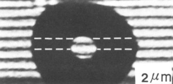
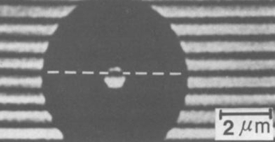
Essential Graduate Physics
QM: Quantum Mechanics
2
,
(3.34b)
B
0
12
12
B 0
' 0
where the fundamental constant 0 ’ 2/ e 4.1410-15 Wb has the meaning of the magnetic flux necessary to change 12 by 2, i.e. to shift the interference pattern (11) by one period, and is called the normal magnetic flux quantum – “normal” because of the reasons we will soon discuss.
(a)
(b)
Fig. 3.3. Typical results of a two-paths interference experiment by A. Tonomura et al., Phys. Rev.
Lett. 56, 792 (1986), showing the AB effect for electrons shielded from the applied magnetic field.
In this particular experimental geometry, the AB effect produces a relative shift of the interference patterns inside and outside the dark ring. (a) = 0 ’/2, (b) = 0 ’. © 1986 APS.
The AB effect may be “almost explained” classically, in terms of Faraday’s electromagnetic induction. Indeed, a change of magnetic flux in time induces a vortex-like electric field E around it. That field is not restricted to the magnetic field’s location, i.e. may reach the particle’s trajectories.
The field’s magnitude (or rather of its integral along the contour C) may be readily calculated by integration of the first of Eqs. (21):
d Φ
V
Δ ΔE d
r
.
(3.35)
dt
C
I hope that in this expression the reader readily recognizes the integral (“undergraduate”) form of Faraday’s induction law.13 To calculate the effect of this electric field on the particles, let us assume that the variable separation described by Eq. (1.57) may be applied to the endpoints 1 and 2 of the particle’s alternative trajectories as two independent systems,14 and that the magnetic flux’ change by a certain amount does not change the spatial factors 1,2, provided that the phases 1,2 are included into the time-dependent factors a 1,2. Then we may repeat the arguments that were used in Sec. 1.6 at the discussion of the Josephson effect, and since the change (35) leads to the change of the potential energy difference U = q V between the two points, we may rewrite Eq. (1.72) as d
U
q
q d
12
V
.
(3.36)
dt
dt
Integrating this relation over the time of the magnetic field’s change, we get
13 See, e.g., EM Sec. 6.1.
14 This assumption may seem a little bit of a stretch, but the resulting relation (37) may be indeed proven for a rather realistic model, though that would take more time/space than I can afford.
Chapter 3
Page 8 of 64
QM: Quantum Mechanics
q
,
(3.37)
12
– superficially, the same result as given by Eq. (34).
However, this interpretation of the AB effect is limited. Indeed, it requires the particle to be in the system (on the way from the source to the detector) during the flux change, i.e. when the induced electric field E may affect its dynamics. On the contrary, Eq. (34) predicts that the interference pattern would shift even if the field change has been made when there was no particle in the system, and hence the field E could not be felt by it. Experiment confirms the latter conclusion. Hence, there is something in the space where a particle propagates (i.e., outside of the magnetic field region), that transfers the information about even the static magnetic field to the particle. The standard interpretation of this surprising fact is as follows: the vector potential A is not just a convenient mathematical tool, but a physical reality (just as its scalar counterpart is), despite the large freedom of choice we have in prescribing specific spatial and temporal dependences of these potentials without affecting any observable – see Eqs. (23)-(24).
To conclude this section, let me briefly discuss the very interesting form taken by the AB effect in superconductivity. To be applied to this case, our results require two changes. The first one is simple: since superconductivity may be interpreted as a result of the Bose-Einstein condensate of Cooper pairs with electric charge q = –2 e, 0 ’ has to be replaced by the so-called superconducting flux quantum 15
Super-
conducting
Φ
07
.
2
10
15 Wb 07
.
2
10 7 Gs cm2.
(3.38)
flux
0
e
quantum
Second, since the pairs are Bose particles and are all condensed in the same (ground) quantum state described by the same wavefunction, the total electric current density, proportional to the probability current density j, may be extremely large – in practical superconducting materials, up to
~1012 A/m2. In these conditions, one cannot neglect the contribution of that current into the magnetic field and hence into its flux , which (according to the Lenz rule of the Faraday induction law) tries to compensate for changes in external flux. To see possible results of this contribution, let us consider a closed superconducting loop (Fig. 4). Due to the Meissner effect (which is just another version of the flux self-compensation), the current and magnetic field penetrate into a superconductor by only a small distance (called the London penetration depth) L ~ 10-7 m.16 If the loop is made of a superconducting
“wire” that is considerably thicker than L, we may draw a contour deep inside the wire, at which the current density is negligible. According to the last form of Eq. (28), everywhere at the contour, q
A 0 .
(3.39)
Integrating this equation along the contour as before (in Fig. 4, from some point 1, all the way around the ring to the virtually coinciding point 2), we need to have the phase difference 12 equal to 2 n, because the wavefunction exp{ i} at the initial and final points 1 and 2 should be “essentially” the same, i.e. produce the same observables. As a result, we get
15 One more bad, though common term: a wire may (super)conduct, but a quantum hardly can!
16 For more detail, see EM Sec. 6.4.
Chapter 3
Page 9 of 64
QM: Quantum Mechanics
Φ A d
r
2 n
.
n
(3.40) Flux
0
q
quantization
C
This is the famous flux quantization effect,17 which justifies the term “magnetic flux quantum” for the constant 0 given by Eq. (38).
B
C
1
2
Fig. 3.4. The magnetic flux quantization in a
superconducting loop (schematically).
Here I have to mention the very interesting effects of “flux semi-quantization” that arise when superconductor loops are closed with Josephson junctions, forming the so-called Superconducting QUantum Interference Devices (“SQUIDs”). Such devices may be used, in particular, for supersensitive magnetometry and ultrafast low-power computing,18 and are currently explored as a possible basis for quantum computation and cryptography – see Sec. 8.5 below.
3.2. Landau levels and quantum Hall effect
In the last section, we have used the Schrödinger equation (27) for an analysis of static magnetic field effects in “almost-1D”, circular geometries shown in Figs. 1, 2, and 4. However, this equation describes very interesting effects in fully higher dimensions as well, especially in the 2D case. Let us consider a quantum particle free to move within the [ x, y] plane only (say, due to its strong confinement in the perpendicular direction z – see the discussion at the beginning of Sec. 2.1). In this case, Eq. (27) reduces to a similar equation but with the Laplace operator acting only in the directions x and y:
2
2
q
n
n
i A
E .
(3.41)
2 m x
x
y
y
Let us find its solutions for the simplest case when the applied static magnetic field is uniform and normal to the motion plane:
B B n .
(3.42)
z
According to the second of Eqs. (21), this relation imposes the following restriction on the choice of the vector potential:
Ay A
x B ,
(3.43)
x
y
17 It was predicted in 1949 by Fritz London and experimentally discovered (independently and virtually simultaneously) in 1961 by two experimental groups: B. Deaver and W. Fairbank, and R. Doll and M. Näbauer.
18 A brief review of these applications, and recommendations for further reading may be found in EM Sec. 6.5.
Chapter 3
Page 10 of 64
QM: Quantum Mechanics
but the gauge transformations still give us a lot of freedom in its choice. The natural axially symmetric form, A = nB/2, where = ( x 2 + y 2)1/2 is the distance from some z-axis, leads to cumbersome math.
In 1930, L. Landau realized that the energy spectrum of Eq. (41) may be obtained by making a much simpler, though very counter-intuitive gauge choice:
A ,
0
A B
(3.44)
x
y
x x 0 ,
(with arbitrary x 0), which evidently satisfies Eq. (43), though ignores the physical symmetry of the x and y directions for the field (42).
Now, expanding the eigenfunction into the Fourier integral in the y-direction:
( x, y) X ( x
) exp
,
(3.45)
k
ik y y 0 dk
we see that for each component of this expansion, Eq. (41) yields a specific equation 2
d
q
2
n
in k B x x
.
(3.46)
0 X EX
x
y
k
k
2 m dx
Since the two vectors inside the curly brackets are mutually perpendicular, its square has no cross-terms, so Eq. (46) reduces to
2 d 2
q 2
2
2
k
X
,
where
.
(3.47)
2
k
B x x ' 0 X
EX
x '
x
2 m dx
2 m
k
k
0
0
q B
But this 1D Schrödinger equation is identical to Eq. (2.261) for a 1D harmonic oscillator,19 with the center at point x 0 ’, and the frequency 0 equal to
q B
.
(3.48)
c
m
In the last expression, it is easy to recognize the cyclotron frequency of the classical particle’s rotation in the magnetic field. (It may be readily obtained using the 2nd Newton law for a circular orbit of radius r, v 2
m
F qv ,
(3.49)
B
B
r
and noting that the resulting ratio v/ r = q B / m is just the radius-independent angular velocity c of the particle’s rotation.) Hence, the energy spectrum for each Fourier component of the expansion (45) is the same:
Landau
1
E
levels
n
,
(3.50)
n
c
2
independent of x 0, y 0, and k.
19 This result may become a bit less puzzling if we recall that at the classical circular cyclotron motion of a particle, each of its Cartesian coordinates, including x, performs sinusoidal oscillations with frequency (48), just as a 1D harmonic oscillator with this frequency.
Chapter 3
Page 11 of 64


Essential Graduate Physics
QM: Quantum Mechanics
Hence, this is a good example of a highly degenerate system: for each eigenvalue En, there are many similarly-structured eigenfunctions that differ by the positions { x 0, y 0} of their centers and the rate k of their phase change along the y-axis. They may be used to assemble a large variety of linear combinations, including 2D wave packets whose centers move along classical circular orbits. Note, however, that the radius of such rotation cannot be smaller than the so-called Landau radius, 1/ 2
1/ 2
r
,
(3.51) Landau
L
radius
mc
B
q
which characterizes the minimum size of the wave packet, and follows from Eq. (2.276) after the replacement 0 c. This radius is remarkably independent of the particle mass, and may be interpreted in the following way: the scale B A min of the applied magnetic field’s flux through the effective area A
2
min = 2 r L of the smallest wave packet is just one normal flux quantum 0 ’ 2/ q .
A detailed analysis of such wave packets (for which we would not have time in this course) proves, in particular, the virtually evident fact: the applied magnetic field does not change the average density dN 2/ dE of different 2D states on the energy scale, given by Eq. (1.92), but just “assembles” the states them on the Landau levels (see Fig. 5a), so the number of different orbital states on each Landau level (per unit area) is
N
1 dN
1
2
dN
d k
1
1
A
1
B
q
2
2
n
Δ
2
E
Δ E
k
(3.52)
L
B 0
2
B 0
A
A dE
A d k
dk dE / dk
A 2 2
.
2
2
k /
c
m
2
This expression may again be interpreted in terms of magnetic flux quanta: n L0 ’ = B, i.e. there is one particular state on each Landau level per each normal flux quantum.
En
B = 0
(a)
(b)
B 0
electrodes
E
c
F
Fig. 3.5. (a) The “assembly” of
2D states on Landau levels, and
(b) filling the levels with
c
electrons at the quantum Hall
effect.
0
The most famous application of the Landau levels picture is the explanation of the quantum Hall effect 20. It is usually observed in the “Hall bar” geometry sketched in Fig. 6, where electric current I is passed through a rectangular conducting sample placed into magnetic field B perpendicular to the sample’s plane. The classical analysis of the effect may be based on the notion of the Lorentz force (14).
As the magnetic field is turned on, this force starts to deviate the effective charge carriers (electrons or holes) from their straight motion between the electrodes, bending them toward the insulated sides of the 20 It was first observed in 1980 by a group led by Klaus von Klitzing, while the classical version (54) of the effect was first observed by Edwin Hall a century earlier – in 1879.
Chapter 3
Page 12 of 64
Essential Graduate Physics
QM: Quantum Mechanics
bar (in Fig. 6, parallel to the x-axis). Here the carriers accumulate, generating a gradually increasing electric field E until its force (16) exactly balances the Lorentz force (14):
E
q
qv
,
(3.53)
y
x B
where vx is the drift velocity of the carriers along the bar (Fig. 6), providing the sustained balance condition E y/ vx = B at each point of the sample.
y
w
E
I
v, j
B
Fig. 3.6. The Hall bar geometry. Darker
rectangles show external (3D) electrodes.
0
x
l
With n 2 carriers per unit area, in a sample of width w, this balance condition yields the following classical expression for the so-called Hall resistance R H, remarkably independent of w and l: Classical
V
E w
Hall
R
y
y
B
.
(3.54)
H
effect
I
qn v w
qn
x
2 x
2
This formula is broadly used in practice for the measurement of the 2D density n 2 of the charge carriers and of the carrier type: electrons with q = – e < 0, or holes with the effective charge q = + e > 0.
However, in experiments with high-quality (low-defect) 2D samples, at sub-kelvin temperatures21 and high magnetic fields, the linear growth of R H with B, described by Eq. (54), is interrupted by virtually horizontal plateaus (Fig. 7).
R
H
Fig. 3.7. A typical record of the integer
quantum Hall effect. The lower trace (with
sharp peaks) shows the diagonal element,
V
x/ Ix, of the resistance tensor. (Adapted from
https://www.nobelprize.org/nobel_prizes/phy
sics/laureates/1998/press.html ).
B
tesla
21 In some systems, such as the graphene (virtually perfect 2D sheets of carbon atoms – see Sec. 4 below), the effect may be more stable to thermal fluctuations, due to their topological properties, so it may be observed even at room temperature – see, e.g., K. Novoselov et al., Science 315, 1379 (2007). Note also that in some spontaneously-magnetized ferromagnetic layers, the quantum Hall effect may be observed in the absence of an external magnetic field – see, e.g., M. Götz et al., Appl. Phys. Lett. 112, 072102 (2018) and references therein.
Chapter 3
Page 13 of 64
QM: Quantum Mechanics
Most remarkably, the experimental values of R H on these plateaus are reproduced with extremely high accuracy (up to ~10-9) from sample to sample.22 They are described by the following formula: 1
2
Quantum
R R ,
where R
,
(3.55)
H
K
K
Hall
2
i
e
effect
with the following value:
R 25.812 807 459
k
304 ,
(3.56)
K
and i is (only until the end of this section, following tradition!) the plateau number, i.e. a real integer.
This effect may be explained using the Landau-level picture. The 2D sample is typically in weak contact with 3D electrodes whose conductivity electrons, at low temperatures, fill all states with energies below a certain Fermi energy E F – see Fig. 5b. According to Eqs. (48) and (50), as B is increased, the spacing c between the Landau levels increases proportionately, so fewer and fewer of these levels are below E F (and hence in equilibrium, all their states are filled), and within certain ranges of field variations, the number i of the filled levels is constant. (In the schematic Fig. 5b, i = 2.) So, plugging n 2 = in L and q = – e into Eq. (54), and using Eq. (52) for n L, we get 1
1 2
R
B
,
(3.57)
H
2
i qn
i e
L
i.e. exactly the experimental result (55).
This admittedly oversimplified explanation of the quantum Hall effect does not take into account at least two important factors:
(i) the nonuniformity of the background potential U( x, y) in realistic Hall bar samples, and the role of the quasi-1D edge channels this nonuniformity produces;23 and
(ii) the Coulomb interaction of the electrons, in high-quality samples leading to the formation of R H plateaus with not only integer but also fractional values of i (1/3, 2/5, 3/7, etc.).24
Unfortunately, a thorough discussion of these very interesting features is well beyond the framework of this course.25,26
22Due to this high accuracy (which is a rare exception in solid-state physics!), the von Klitzing constant R K was used in metrology for the “legal” ohm’s definition. Since 2018, the values of and e, and hence of R K, are considered exactly known and fixed – see Appendix UCA: Selected Units and Constants.
23 Such quasi-1D regions, with the width of the order of r L, form along the lines where the Landau levels cross the Fermi surface and are actually responsible for all the electron transfer at the quantum Hall effect (giving the pioneering example of what is nowadays called the topological insulators). The particle motion along these channels is effectively one-dimensional; because of this, it is unaffected by modest unintentional nonuniformities of the potential U( x, y). This fact is responsible for the extraordinary accuracy of Eq. (55).
24 This fractional quantum Hall effect was discovered in 1982 by D. Tsui, H. Stormer, and A. Gossard. In contrast, the effect described by Eq. (55) with integer i (Fig. 7) is now called the integer quantum Hall effect.
25 For a comprehensive discussion of these effects, I can recommend either the monograph by D. Yoshioka, The Quantum Hall Effect, Springer, 1998, or the review by D. Yennie, Rev. Mod. Phys. 59, 781 (1987). (See also the later publications cited above.)
26 Note also that the quantum Hall effect is sometimes discussed in terms of the so-called Berry phase, one of the geometric phases – the notion apparently pioneered by S. Pancharatnam in 1956. However, in the “usual”
quantum Hall effect the Berry phase equals zero, and I believe that this concept should be saved for the discussion of more topologically involved systems. Unfortunately, I will have no time/space for a discussion of such systems Chapter 3
Page 14 of 64
QM: Quantum Mechanics
3.3. Scattering and diffraction
The second class of quantum effects that become richer in multi-dimensional spaces, is typically referred to as either diffraction or scattering – depending on the context. In classical physics, these two terms are used to describe very different effects. The term “diffraction” is used for the interference of the waves re-emitted by elementary components of extended objects, under the effect of a single incident wave.27 On the other hand, the term “scattering” is used in classical mechanics to describe the result of the interaction of a beam of particles 28 incident upon an object called the scatterer – see Fig. 8.
1
r
a,
k
detector
k
a
k i
scattered particles
incident
scatterer
Fig. 3.8. Scattering (schematically).
particles
Most commonly, the detector of the scattered particles is located at a large distance r >> a from the scatterer. In this case, the main observable independent of r is the flux (the number per unit time) of particles scattered in a certain direction, i.e. their flux per unit solid angle . Since it is proportional to the incident flux of particles per unit area, the efficiency of scattering in a particular direction may be characterized by the ratio of these two fluxes. This ratio is called the differential cross-section of the scatterer:
Differential
d
of
flux
angle
solid
unit
per
particles
scatterd
cross-
.
(3.58)
section
d
of
flux
area
unit
per
particles
incident
Such terminology and notation stem from the fact that the integral of d/ d over all scattering angles, Total
d
of
flux
total
particles
scattered
cross-
Ω
section
d
,
(3.59)
Ω
d
area
unit
per
per
flux
incident
evidently having the dimensionality of area, has a simple interpretation as the total cross-section of scattering. For the simplest case when a solid object scatters all classical particles hitting its surface but does not affect the particles flying by it, is just the geometric area of the scatterer, as observed from the direction of the incident particles. In classical mechanics, we first calculate the particle’s scattering angle as a function of its impact parameter b and then average the result over all values of b, considered random. 29
in this course, and have to refer the interested reader to special literature – see, e.g., either the key original papers collected by A. Shapere and F. Wilczek, Geometric Phases in Physics, World Scientific, 1992, or the monograph by A. Bohm et al., The Geometric Phase in Quantum Systems, Springer, 2003.
27 The notion of interference is very close to diffraction, but the former term is typically reserved for the wave re-emission by just a few components, such as two slits in the Young experiment – see Figs. 1 and 2. A detailed discussion of diffraction and interference of electromagnetic waves may be found in EM Secs. 8.3-8.8.
28 In the classical wave theory, the term “scattering” is typically reserved for wave interaction with disordered sets of small objects – see, e.g., EM Sec. 8.3.
29 See, e.g., CM Sec. 3.5.
Chapter 3
Page 15 of 64
QM: Quantum Mechanics
In quantum mechanics, due to the particle/wave duality, a relatively broad, parallel beam of incident particles of the same energy E may be fairly represented with a plane de Broglie wave (1.88):
exp i
,
(3.60)
i
i
k r
i
with the free-space wave number k i = k = (2 mE)1/2/. As a result, the particle scattering becomes a synonym of the de Broglie wave diffraction, and (somewhat counter-intuitively) the description of the effect becomes simpler, excluding the notion of the impact parameter. Indeed, the wave (60) corresponds to a constant probability current density (1.49):
2
j
k ,
(3.61)
i
i
i
m
which is exactly the flux of incident particles per unit area that is used in the denominator of Eq. (58), while the numerator of that fraction may be simply expressed via the probability current density js of the scattered de Broglie waves:
2
d
j r
s
,
at r .
a
(3.62)
d
j i
Hence the task of finding d/ d is reduced to the calculation of j s at sufficiently large distances r from the scatterer. For the elastic scattering (when the energy E of the scattered particles is the same as that of the incident particles) this may be done by solving the stationary Schrödinger equation (1.65).
Let us rewrite it in the form
2
2
2
k 2
E H ˆ
r
,
(3.63)
0
U ( ) ,
H ˆ
with
and
,
E
0
2 m
2 m
where the potential energy U(r) describes the scatterer’s effect. Looking for the solution of Eq. (62) in the natural form
,
(3.64)
i
s
where i is the incident wave (60) and s has the sense of the scattered wave, and taking into account that the former wave satisfies the free-space Schrödinger equation
ˆ
H E ,
(3.65)
0
i
i
we may reduce Eq. (63) to either of the following equivalent forms:
m
2
2
2
ˆ
E H
U r
k
U r
.
(3.66)
0 s
i
s ,
(
)
s
2
For applications, an integral version of this equation is frequently more convenient. To derive it, we may look at the second of Eqs. (66) as a linear inhomogeneous differential equation for the function
s, thinking of its right-hand side as a known “source”. The solution of such an equation obeys the linear superposition principle, i.e. we may represent it as the sum of the waves outcoming from all elementary volumes d 3 r’ of the scatterer. Mathematically, this sum may be expressed as either 2 m
(r)
U ( '
r ) ( '
r G
) (r, '
r ) d 3 r' ,
(3.67a)
s
2
Chapter 3
Page 16 of 64
QM: Quantum Mechanics
or, equivalently, as30
2 m
(r) r
(r ) (r ) (r, r )
,
(3.67b)
i
U '
' G
' d 3 r'
2
where G(r, r ’) is the spatial Green’s function, defined as such an elementary, spherically symmetric response of the 3D Helmholtz equation to a point source, i.e. the outward-propagating solution of the following equation31
2
2
k G (r ' r) .
(3.68)
But we already know such a solution of this equation – see Eq. (7) and its discussion: f
G r
( , '
r ) eikR ,
where R
r '
r ,
(3.69)
R
so we need just to calculate the coefficient f+ for Eq. (68). This can be done in several ways, for example by noticing that at R << k-1, the second term on the left-hand side of Eq. (68) is negligible, so it is reduced to the well-known Poisson equation with a delta-functional right-hand side, which describes, for example, the electrostatic potential induced by a point electric charge. Either recalling the Coulomb law or applying the Gauss theorem,32 we readily get the asymptote
1
G
,