

Quantum Mechanics by Konstantin K. Likharev - HTML preview
Download the book in PDF, ePub, Kindle for a complete version.
(2.135)
scatterer
i
1 i
As a sanity check, Eq. (128) applied to this result, immediately brings us back to Eq. (79).
The next example may seem strange at first glance: what if there is no scatterer at all between points x 1 and x 2? If the points coincide, the answer is indeed trivial and can be obtained, e.g., from Eq.
(135) by taking W = 0, i.e. = 0:
1 0
Identity
T
I
(2.136)
transfer
0
matrix
0 1
– the so-called identity matrix. However, we are free to choose the reference points x 1,2 participating in Eq. (120) as we wish. For example, what if x 2 – x 1 = a? Let us first take the forward-propagating wave alone: B 2 = 0 (and hence B 1 = 0); then
ik( x x )
ik( x x ) ik( x x )
1
2
1
2
A e
A e
e
.
(2.137)
2
1
1
1
The comparison of this expression with the definition (120) for j = 2 shows that A 2 = A 1 exp{ ik( x 2 – x 1)}
= A 1 exp{ ika}, i.e. T 11 = exp{ ika}. Repeating the calculation for the back-propagating wave, we see that T 22 = exp{– ika}, and since the space interval provides no particle reflection, we finally get Transfer
matrix:
ika
e
0
spatial
T
,
(2.138)
a
interval
ika
0
e
independently of a common shift of points x 1 and x 2. At a = 0, we naturally recover the special case (136).
Chapter 2
Page 29 of 76
QM: Quantum Mechanics
Now let us use these simple results to analyze the double-barrier system shown in Fig. 15. We could of course calculate its properties as before, writing down explicit expressions for all five traveling waves symbolized by arrows in Fig. 15, then using the boundary conditions (124) and (125) at each of the points x 1,2 to get a system of four linear equations, and finally, solving it for four amplitude ratios.
a
W x x
W x x 2
1
E
Fig. 2.15. The double-barrier system. The
dashed lines show (schematically) the quasi-
levels of the metastable-state energies.
x
x
x
1
2
However, the transfer matrix approach simplifies the calculations, because we may immediately use Eqs. (132), (135), and (138) to write
1 i
i eika
0 1 i
i
T T T T
.
(2.139)
a
ika
i
1 i 0
e
i
1 i
Let me hope that the reader remembers the “row by column” rule of the multiplication of square matrices;30 using it for the last two matrices, we may reduce Eq. (139) to
1 i
i 1
(
ika
i ) e
ika
i e
T
.
(2.140)
ika
ika
i
1 i i e
1
( i ) e
Now there is no need to calculate all elements of the full product T, because, according to Eq. (128), for the calculation of the barrier’s transparency T we need only one of its elements, T 11: 1
1
Double
T
.
(2.141) barrier:
2
2
2
T
ika
ika
transparency
11
e
1
( i )2 e
This result describes oscillations of the transparency: at a fixed parameter , T is a -periodic function of the product ka, reaching its maximum (T = 1) at some point of each period – see Fig. 16a.
Indeed, the denominator in Eq. (141) may be interpreted as the squared length of the difference between two 2D vectors, one of length 2 and another of length (1 – i)2 = 1 + 2, with the angle = 2 ka +
const between them – see Fig. 16b. At the resonance, the vectors are aligned, and their difference is smallest (equal to 1) so Tmax = 1. (This result is exact only if the two barriers are exactly equal.) This means that, rather counter-intuitively, the maximum transparency of the system is perfect even at >> 1, i.e. in the case of a very low transparency of each of the component barriers. This is the famous resonant tunneling effect.31
N
30 In the analytical form: AB
A B , where N is the square matrix rank (in our current case, N = 2).
jj'
jj" j"j'
j" 1
31 In older literature, it is sometimes called the Townsend (or “Ramsauer-Townsend”) effect. However, nowadays it is more common to use the last term only for a similar effect at 3D scattering – to be discussed in Chapter 3.
Chapter 2
Page 30 of 76
QM: Quantum Mechanics
(a)
(b)
2
3
.
0
Im
1
0.8
1
2
1
0.6
T
k
k
0
Re
0.4
0
.
1
Fig. 2.16. Resonant tunneling through a
0.2
potential well with delta-functional walls:
0
.
3
(a) the system’s transparency as a
0
function of ka, and (b) calculating the
0
0.5
1
1.5
2
ka /
resonance’s FWHM at >> 1.
Its physics is the constructive interference of de Broglie waves, similar to that of electromagnetic waves (for example, light) in a Fabry-Perot resonator formed by two parallel semi-transparent mirrors.32 Namely, the incident de Broglie wave may be thought to undertake, on its way through the system, several sequential reflections from these semi-transparent walls. At k = kn, i.e. at 2 ka = 2 kna =
2 n, the phase differences between all these partial waves are multiples of 2, so they add up in phase –
“constructively”. (At large but finite , the resonance condition slightly deviates from ka = n.) Note that the same constructive interference of numerous reflections from the walls may be used to interpret the standing-wave eigenfunctions (1.84), so the resonant tunneling at >> 1 in our current system may be also considered a result of the resonant induction of such a standing wave, with a very large amplitude, in the space between the barriers, with the transmitted wave’s amplitude proportionately increased.
The resonance peaks of the transparency may be very narrow. Their so-called FWHM (the common acronym for the Full Width at Half-Maximum), for the most interesting case for >> 1, may readily calculated by using the same vector diagram shown in Fig. 16b. By definition, FWHM is the difference k = k+ – k– between such two values of k, on the opposite slopes of the same resonance curve, at that T = Tmax/2 – see the arrows in Fig. 16a. Let the two vectors in Fig. 16b be misaligned by a small angle << 1, so the length of the difference vector is much smaller than 2. To double its length squared, and hence to reduce T by a factor of two in comparison with its maximum value of 1, the arc between the vectors, equal to 2 , should also become equal to 1, i.e. 2(2 k a + const) to become equal to 1. Subtracting these two equalities from each other, we get
1
k k k
k .
(2.142)
2
a
Now let us use the simple system shown in Fig. 15 to discuss an issue of large conceptual significance. For that, consider what would happen if at some initial moment (say, t = 0) we placed a 1D
quantum particle inside the double-barrier well with >> 1, and left it there alone, without any incident wave. To simplify the analysis, let us assume that the initial state of the particle coincides with one of the stationary states of the infinite-wall well of the same size – see Eq. (1.84): 32 See, e.g., EM Sec. 7.9. Note also that as Eqs. (2.71) and Fig. 7 show, similar resonant tunneling takes place on the top of the rectangular barrier of height U 0 < E, thanks to the step-down reflection from its borders.
Chapter 2
Page 31 of 76
QM: Quantum Mechanics
2 1/2
n
( x )
0
, ( x)
.
(2.143)
n
sin k ( x x )
k
n
n
1 ,
where
,
,
1 ,...
2
a
n
a
At , this is just an eigenstate of the system, and from our analysis in Sec. 1.5 we know the time evolution of its wavefunction:
2 1/2
E
k 2
( x, t) ( x) exp
sin
( ) exp ,
with
, (2.144)
n
i tn
k x x
n
1
i tn
n
n
a
n
2 m
telling us that the particle remains in the well at all times with a constant probability: W( t) = W(0) = 1.
However, if the parameter is large but finite, the de Broglie wave would slowly “leak out”
from the well, so W( t) would slowly decrease. Such a state is called metastable. Let us derive the law of its time evolution, assuming that at the slow leakage, with a characteristic time >> 1/ n, does not affect the instant wave distribution inside the well, besides the gradual, slow reduction of W.33 Then we can generalize Eq. (144) as
W
2 1/ 2
( x, t)
sin k ( x x ) exp
exp
exp
, (2.145)
n
1
i tn A i k x
t
n
n
B
i k x
t
n
n
a
making the probability of finding the particle in the well equal to some W 1. As the last form of Eq.
(145) shows, this is the sum of two traveling waves, with equal magnitudes of their amplitudes and hence equal but opposite probability currents (5):
1/ 2
W
W n
A B
,
2
I
A k
,
I I .
(2.146)
2
A
n
a
m
m 2
B
A
a a
But we already know from Eq. (79) that at >> 1, the delta-functional wall’s transparency T equals 1/2, so the wave carrying the current IA, incident on the right wall from the inside, induces an outcoming wave outside of the well (Fig. 17) with the following probability current: 1
1 n W
I I
T
I
.
(2.147)
R
A
2
A
2
2
2 ma
~ v
gr
I
I
L
R
E 1
v t
0
v t
x
gr
gr
Fig. 2.17. A schematic snapshot of the wavefunction (say, Re) in the simple model shown in Fig. 15, at time t > >> 1/1 after the particle’s placement into the lowest metastable state with energy E 1.
Absolutely similarly,
1
I
I I .
(2.148)
L
2
B
R
33 This (virtually evident) assumption finds its formal justification in the perturbation theory to be discussed in Chapter 6.
Chapter 2
Page 32 of 76
QM: Quantum Mechanics
Now we may combine the 1D version (6) of the probability conservation law for the well’s interior: dW
I I 0 ,
(2.149)
R
L
dt
with Eqs. (147)-(148) to write
dW
1 n
W .
(2.150)
dt
2
ma 2
This is just the standard differential equation,
Metastable
dW
1
state:
W ,
(2.151)
decay law
dt
of an exponential decay, W( t) = W(0)exp{- t/}, where the constant is called the metastable state’s lifetime. In our particular case,
2
ma
2
,
(2.152)
n
.
Using Eq. (2.33b) for the de Broglie waves’ group velocity, for our particular wave vector giving v gr = kn/ m = n/ ma, Eq. (152) may be rewritten in a more general form, Metastable
t
state:
a
,
(2.153)
lifetime
T
where the attempt time t a is equal to a/ v gr, and (in our particular case) T = 1/2. Eq. (153) is valid for a broad class of similar metastable systems;34 it may be interpreted in the following semi-classical way.
The particle travels back and forth between the confining potential barriers, with the time interval t a between the sequential moments of incidence, each time attempting to leak through the wall, with the success probability equal to T, so the reduction of W per each incidence is W = – W T. In the limit T << 1, this equality immediately leads to the decay equation (151) with the lifetime (153).
Another useful look at Eq. (152) may be taken by returning to the resonant tunneling problem in the same system, and expressing the resonance width (142) in terms of the incident particle’s energy: 2
2
2
2
2
k k
k
n
n
1
n
E
k
.
(2.154)
2
2
2
2 m
m
m
a
ma
Comparing Eqs. (152) and (154), we get a remarkably simple, parameter-independent formula35
Energy-time
uncertainty
E .
(2.155)
relation
34 Essentially the only requirement for the attempt time t a is to be much longer than the effective time (the so-called instanton time, see Sec. 5.3 below) of tunneling through the barrier. In the delta-functional approximation for the barrier, the latter time vanishes, so that this requirement is always fulfilled.
35 Note that Eq. (2.151) may be formally obtained from the basic Schrödinger equation (1.61) by adding an imaginary part, equal to (– E/2), to its eigenenergy En. Indeed, in this case Eq. (1.62) becomes an( t) =
const exp{ –i( En – i E/2} t/} const exp{ -iEnt/}exp{ - Et/2} = const exp{ -iEnt/}exp{ -t/2}, so that W( t) an( t)2 exp{ -t/}. Such formalism, which hides the physical origin of the state’s decay, may be convenient for some calculations, but misleading in other cases, and I will not use it in this course.
Chapter 2
Page 33 of 76
QM: Quantum Mechanics
This energy-time uncertainty relation is certainly more general than our simple model; for example, it is valid for the lifetime and resonance tunneling width of any metastable state in the potential profile of any shape. This seems very natural since because of the energy identification with frequency, E = , pertinent to quantum mechanics, Eq. (155) may be rewritten as = 1 and seems to follow directly from the Fourier transform in time, just as the Heisenberg’s uncertainty relation (1.35) follows from the Fourier transform in space. In some cases, even those not involving any state decay, these two relations are indeed interchangeable. For example, Eq. (24) for the Gaussian wave packet width may be rewritten as E t = , where E = ( d/ dk) k = v gr k is the r.m.s. spread of energies of monochromatic components of the packet, while t x/ v gr is the time scale of the packet’s passage through a fixed observation point x.
However, Eq. (155) is much less general than Heisenberg’s uncertainty relation (1.35). Indeed, the Cartesian coordinates of a particle, the Cartesian components of its momentum, and the energy E are regular observables, represented by operators. In contrast, in the non-relativistic quantum mechanics we are studying now, time is treated as a c-number argument, and is not represented by an operator, so Eq.
(155) cannot be derived in such general assumptions as Eq. (1.35). Thus the time-energy uncertainty relation should be used with caution. Unfortunately, not everybody is so careful. One can find, for example, claims that due to this relation, the energy of a system cannot be measured, during a time
interval t, with an accuracy better than / t. These claims are wrong.36 Another incorrect statement is that the energy dissipated by any system performing an elementary (single-bit) calculation during a time interval t has to be larger than / t.37
Now that we have a quantitative mathematical description of the metastable state’s decay (valid, again, only at >> 1, i.e. at >> t a), we may use it to discuss two important conceptual issues of quantum mechanics. First, the decay is one of the simplest examples of systems that may be considered, from two different points of view, as either Hamiltonian (and hence time- reversible), or open (and hence irreversible). Indeed, from the former point of view, our particular system is certainly described by a time-independent Hamiltonian (1.41), with the potential energy
U x W x x x x (2.156)
1
2
– see Fig. 15 again. In this point of view, the total probability of finding the particle somewhere on the x-axis remains equal to 1, and the full system’s energy, calculated from Eq. (1.23),
E
*
x t H ˆ
,
x, t d 3 x
,
(2.157)
remains constant. On the other hand, since the “emitted” wave packets would never return to the potential well,38 it makes much sense to look at the well’s region alone. For such a truncated, open 36 See, e.g., V. Braginsky and F. Khalili, Quantum Measurement, Cambridge U. Press, 1992.
37 Here I dare to refer to my own old work K. Likharev , Int. J. Theor. Phys. 21, 311 (1982), which provided a constructive proof (for a particular system) that at reversible computations, whose idea had been put forward in 1973 by C. Bennett (see, e.g., SM Sec. 2.3), energy dissipation may be lower than this apparent “quantum limit”.
38 For more realistic 2D and 3D systems, this statement is true even if the system as a whole is confined inside some closed volume, much larger than the potential well housing the metastable states. Indeed, if the walls providing such confinement are even slightly uneven, the emitted plane-wave packets will be reflected from them, but would never return to the well intact. (See SM Sec. 2.1 for a more detailed discussion of this issue.) Chapter 2
Page 34 of 76
QM: Quantum Mechanics
system (for which the space beyond the interval [ x 1, x 2] serves as its environment), the probability W of finding the particle inside this interval, and hence its energy E = WEn, decay exponentially per Eq.
(151) – the decay equation typical for irreversible systems. We will return to the discussion of the dynamics of such open quantum systems in Chapter 7.
Second, the same model enables a preliminary discussion of one important aspect of quantum measurements. As Eq. (151) and Fig. 17 show, at t >> , the well becomes virtually empty ( W 0), and the whole probability is localized in two clearly separated wave packets with equal amplitudes, moving from each other with speed v gr, each “carrying the particle away” with a probability of 50%. Now assume that an experiment has detected the particle on the left side of the well. Though the formalisms suitable for quantitative analysis of the detection process will not be discussed until Chapter 7, due to the wide separation x = 2 v gr t >> 2 v gr of the packets, we may safely assume that such detection may be done without any actual physical effect on the counterpart wave packet.39 But if we know that the particle has been found on the left side, there is no chance of finding it on the right side. If we attributed the full wavefunction to all stages of this particular experiment, this situation might be rather confusing.
Indeed, that would mean that the wavefunction at the right packet’s location should instantly turn into zero – the so-called wave packet reduction (or “collapse”) – a hypothetical irreversible process that cannot be described by the Schrödinger equation for this system, even including the particle detectors.
However, if (as was already discussed in Sec. 1.3) we attribute the wavefunction to a certain statistical ensemble of similar experiments, there is no need to involve such artificial notions. The two-wave-packet picture we have calculated (Fig. 17) describes the full ensemble of experiments with all systems prepared in the initial state (143), i.e. does not depend on the particle detection results. On the other hand, the “reduced packet” picture (with no wave packet on the right of the well) describes only a sub-ensemble of such experiments, in which the particles have been detected on the left side. As was discussed in classical examples in Sec. 1.3, for such a redefined ensemble, the probability distribution may be rather different. So, the “wave packet reduction” is just a result of a purely accounting decision of the observer.40 I will return to this important issue in Sec. 10.1 – on the basis of the forthcoming discussion of open systems in Chapters 7 and 8.
2.6. Localized state coupling, and quantum oscillations
Now let us discuss one more effect specific to quantum mechanics. Its mathematical description may be simplified using a model potential consisting of two very short and deep potential wells. For that, let us first analyze the properties of a single well of this type (Fig. 18), which may be modeled similarly to the short and high potential barrier – see Eq. (74), but with a negative “weight”: U x W x,
with W 0 .
(2.158)
In contrast to its tunnel-barrier counterpart (74), such potential sustains a stationary state with a negative eigenenergy E < 0, and a localized eigenfunction , with 0 at x .
39 This argument is especially convincing if the particle’s detection time is much shorter than the time tc = 2 v gr t/ c, where c is the speed of light in vacuum, i.e. the maximum velocity of any information transfer.
40 “The collapse of the wavefunction after measurement represents nothing more than the updating of that scientist’s expectations.” N. D. Mermin, Phys. Today, 72, 53 (Jan. 2013).
Chapter 2
Page 35 of 76
QM: Quantum Mechanics
U ( x)
0
W
( x)
x
E 0
Fig. 2.18. Delta-functional
potential well and its localized
1/ 1/
eigenstate (schematically).
Indeed, at x 0, U( x) = 0, so the 1D Schrödinger equation is reduced to the Helmholtz equation (1.83), whose localized solutions with E < 0 are single exponents vanishing at large distances:41
Ae x for
,
x ,
0
2
2
( x) x
E .
(2.159)
0
with
,
0
Ae x for
,
x ,
0
2 m
Here the pre-exponential coefficients are taken equal to satisfy the boundary condition (76) of the wavefunction’s continuity at x = 0. Plugging Eq. (159) into the second boundary condition, given by Eq.
(75) but now with the negative sign before W, we get
2 m
A
A
W
A ,
(2.160)
2
in which the common factor A 0 may be canceled. This equation42 has one solution for any W > 0: m
W
,
(2.161)
0
2
and hence the system has only one localized state, with the following eigenenergy:43
2
2
2
0
W
m
E E
.
(2.162)
0
2 m
2 2
Now we are ready to analyze the localized states of the two-well potential shown in Fig. 19:
a
a
U ( x) W x x ,
with W 0
.
(2.163)
2
2
Here we may still use the single-exponent solutions similar to Eq. (159), for the wavefunction outside the interval [- a/2, + a/2], but inside the interval, we need to take into account both possible exponents: x
x
a
a
C e
C e
C sinh x
C cosh x
,
for
x ,
(2.164)
A
S
2
2
with the parameter defined as in Eq. (159). The latter of these two equivalent expressions is more convenient because due to the symmetry of the potential (163) with respect to the central point x = 0, the system’s eigenfunctions should be either symmetric (even) or antisymmetric (odd) functions of x (see 41 See Eqs. (56)-(58), with U 0 = 0.
42 Such algebraic equations are frequently called characteristic.
43 Note that this E 0 is equal, by magnitude, to the constant E 0 that participates in Eq. (79). Note also that this result was actually already obtained, “backward”, in the solution of Problem 1.12(ii), but that solution did not address the issue of whether the calculated potential (158) could sustain any other localized eigenstates.
Chapter 2
Page 36 of 76
QM: Quantum Mechanics
Fig. 19), so they may be analyzed separately, only for one half of the system, say x 0, and using just one of the hyperbolic functions (164) in each case.
a / 2 U x
a / 2
0
x
S
E A
Fig. 2.19. A system of two coupled
E
potential wells, and its localized
S
A
eigenstates (schematically).
For the antisymmetric eigenfunction, Eqs. (159) and (164) yield
a
sinh x
,
0
for
x ,
C
2
(2.165)
A
A
a
a
a
sinh
exp x , for x
,
2
2
2
where the front coefficient in the lower line is adjusted to satisfy the condition (76) of the wavefunction’s continuity at x = + a/2 – and hence at x = – a/2. What remains is to satisfy the condition (75), with a negative sign before W, for the derivative’s jump at that point. This condition yields the following characteristic equation:
a
a
2 mW
a
a
a
0
sinh
cosh
sinh
,
1
i.e. coth
2
,
(2.166)
2
2
2
2
2
a
where the 0, given by Eq. (161), is the value of for a single well, i.e. the reciprocal spatial width of its localized eigenfunction – see Fig. 18.
Figure 20a shows both sides of Eq. (166) as functions of the dimensionless product a, for several values of the parameter 0 a, i.e. of the normalized distance between the two wells. The plots show, first of all, that as the parameter 0 a is decreased, the left-hand side and right-hand side plots cross (i.e. Eq. (166) has a solution) at lower and lower values of a. At a << 1, the left-hand side of the last form of this equation may be approximated as 2/ a. Comparing this expression with the right-hand side, we see that this transcendental characteristic equation has a solution (i.e. the system has an antisymmetric localized state) only if 0 a > 1, i.e. if the distance a between the two narrow potential wells is larger than the following value,
2
1
a
,
(2.167)
min
0
W
m
which is equal to the characteristic spread of the wavefunction in a single well – see Fig. 18. (At a
a min, a 0, meaning that the state’s localization becomes weaker and weaker.) In the opposite limit of large distances between the potential wells, i.e. 0 a >> 1, Eq. (166) shows that a >> 1 as well, so its left-hand side may be approximated as 2(1 + exp{ – a}), and the equation yields
Chapter 2
Page 37 of 76
QM: Quantum Mechanics
5
5
4
4
A
S
3
3
LHS (166)
(172)
LHS
2
5
.
1
2
0
.
1
5
.
1
1 a 5
.
0
1
0
RHS
0
.
1
a 5
.
0
0
RHS
0
0
0
1
2
3
a
0
1
2
3
a
Fig. 2.20. Graphical solutions of the characteristic equations of the two-well system, for: (a) the antisymmetric eigenstate (165), and (b) the symmetric eigenstate (171).
1 exp a .
(2.168)
0
0 0
This result means that the eigenfunction is an antisymmetric superposition of two virtually unperturbed wavefunctions (159) of each partial potential well:
1
a
a
x
x x
x x
x x
,
(2.169)
A
R L ,
with R 0 ,
L
0
2
2
2
where the front coefficient is selected in such a way that if the eigenfunction 0 of each well is normalized, so is A. Plugging the middle (more exact) form of Eq. (168) into the last of Eqs. (159), we can see that in this limit the antisymmetric state’s energy is slightly higher than the eigenenergy E 0 of a single well, given by Eq. (162):
2
2
m
E E
a E
W
a .
(2.170)
A
0 1
2
exp
0
,
where
0
exp
2
0
0
The s ymmetric eigenfunction has a form similar to Eq. (165), but is still different from it:
a
cosh x
,
0
for
x ,
C
2
(2.171)
S
S
a
a
a
cosh
exp x , for x
,
2
2
2
giving a characteristic equation similar in structure to Eq. (166), but with a different left-hand side: a
a
0
1 tanh
2
.
(2.172)
2
a
Figure 20b shows both sides of this equation for several values of the parameter 0 a. It is evident that in contrast to Eq. (166), Eq. (172) has a unique solution (and hence the system has a localized symmetric eigenstate) for any value of the parameter 0 a, i.e. for any distance between the partial wells. In the limit of very close wells (i.e. their strong coupling), 0 a << 1, we get a << 1, tanh( a/2) 0, and Eq. (172) yields 20, leading to a four-fold increase of the eigenenergy’s magnitude in comparison with that of the single well:
Chapter 2
Page 38 of 76
QM: Quantum Mechanics
m(2 W )2
E 4 E
,
for a 1.
(2.173)
S
0
2 2
0
The physical meaning of this result is very simple: two very close potential wells act (on the symmetric eigenfunction only!) together, so their “weights” W U( x) dx just add up.
In the opposite, weak coupling limit, i.e. for 0 a >> 1, Eq. (172) shows that a >> 1 as well, so its left-hand side may be approximated as 2(1 – exp{ – a}), and the equation yields
1 exp a .
(2.174)
0
0 0
In this limit, the eigenfunction is a symmetric superposition of two virtually unperturbed wavefunctions (159) of each partial potential well:
1
,
(2.175)
S x
R x L x
2
and the eigenenergy is also close to the energy E 0 of each partial well, but is slightly lower than it: E E
a E
E E
,
(2.176)
S
0 1
2
exp 0
,
that
so
2
0
A
S
where is again given by the last of Eqs. (170).
So, the eigenenergy of the symmetric state is always lower than that of the antisymmetric state.
The physics of this effect (which remains qualitatively the same in more complex two-component systems, most importantly in diatomic molecules such as H2) is evident from the sketch of the wavefunctions A and S, given by Eqs. (165) and (171), in Fig. 19. In the antisymmetric mode, the wavefunction has to vanish at the center of the system, so each its half is squeezed into one half of the system’s spatial extension. Such a squeeze increases the function’s gradient, and hence its kinetic energy (1.27), and hence its total energy. On the contrary, in the symmetric mode, the wavefunction effectively spreads into the counterpart well. As a result, it changes in space slower, and hence its kinetic energy is also lower.
Even more importantly, the symmetric state’s energy level goes down as the distance a is decreased, corresponding to the effective attraction of the partial wells. This is a good toy model of the strongest (and most important) type of atomic cohesion – the covalent (or “chemical”) bonding.44 In the simplest case of the H2 molecule, each of two electrons of the system, in its ground state,45 reduces its kinetic energy by spreading its wavefunction around both hydrogen nuclei (protons), rather than being confined near one of them – as it had to be in a single atom. The resulting bonding is very strong: in chemical units, it is close to 430 kJ/mol, i.e. to 4.5 eV per molecule. Perhaps counter-intuitively, this quantum-mechanical bonding may be even stronger than the strongest classical ( ionic) bonding due to electron transfer between atoms, leading to the Coulomb attraction of the resulting ions. (For example, the atomic cohesion in the NaCl molecule is 4.25 eV.)
44 Historically, the development of the quantum theory of such bonding in the H2 molecule (by Walter Heinrich Heitler and Fritz Wolfgang London in 1927) was the breakthrough decisive for the acceptance of the then-emerging quantum mechanics by the community of chemists.
45 Due to the opposite spins of these electrons, the Pauli principle allows them to be in the same orbital ground state – see Chapter 8.
Chapter 2
Page 39 of 76
QM: Quantum Mechanics
Now let us analyze the dynamic properties of our model system (Fig. 19) carefully because such a pair of weakly coupled potential wells is our first example of the very important class of two-level systems.46 It is easiest to do in the weak-coupling limit 0 a >> 1, when the simple results (168)-(170) and (174)-(176) are quantitatively valid. In particular, Eqs. (169) and (175) enable us to represent the quasi-localized states of the particle in each partial well as linear combinations of its two eigenstates: 1
1
,
.
(2.177)
R x
S x A x
L x
S x A x
2
2
Let us perform the following thought (“gedanken”) experiment: place a particle, at t = 0, into one of these quasi-localized states, say R( x), and leave the system alone to evolve, so 1
( x )
0
, ( x)
x x .
(2.178)
R
( )
( )
S
A
2
According to the general solution (1.69) of the Schrödinger equation, the time dynamics of this wavefunction may be obtained simply by multiplying each eigenfunction by the corresponding complex-exponential time factor:
1
E S
E A
( x, t)
( x) exp
( )exp
.
(2.179)
S
i
t
x
A
i
t
2
From here, using Eqs. (170) and (176), and then Eqs. (169) and (175) again, we get 1
i t
i t
iE t
( x, t)
( x)exp ( x)exp
exp
0
2
S
A
(2.180)
t
t
E t
( x)cos
i ( x)sin
exp
0
i
.
R
L
This result implies, in particular, that the probabilities W R and W L to find the particle, respectively, in the right and left wells change with time as
t
t
W cos2
,
W sin2
,
(2.181) Quantum
R
L
oscillations
mercifully leaving the total probability constant: W R + W L = 1. (If our calculation had not passed this sanity check, we would be in big trouble.)
This is the famous effect of quantum oscillations 47 of the particle’s wavefunction between two coupled localized states, with the frequency
2
E E
A
S
.
(2.182)
In its last form, this result does not depend on the assumption of weak coupling, though the simple form (181) of the oscillations, with its 100% probability variations, does. (Indeed, at a strong coupling of two 46 As we will see later in Chapter 4, these properties are similar to those of spin-½ particles; hence two-level systems are sometimes called spin-½-like systems.
47 Sometimes they are called the Bloch oscillations, but more commonly the last term is reserved for a related but different effect in spatially-periodic systems – to be discussed in Sec. 8 below.
Chapter 2
Page 40 of 76
QM: Quantum Mechanics
subsystems, the very notion of the quasi-localized states R and L is ambiguous.) Qualitatively, this effect may be interpreted as follows: the particle placed into one of the potential wells tries to escape from it via tunneling through the potential barrier separating the wells. (In our particular system shown in Fig. 19, the barrier is formed by the spatial segment of length a, which has the potential energy, U =
0, higher than the eigenstate energy – E 0.) However, in the two-well system, the particle can only escape into the adjacent well. After the tunneling into that counterpart well, the particle tries to escape from it, and hence comes back, etc. – very much as a classical 1D oscillator, initially deflected from its equilibrium position, at negligible damping.
Some care is required in using such interpretation for quantitative conclusions. In particular, let us compare the period T 2/ of the oscillations (181) with the metastable state’s lifetime discussed in the previous section. For our particular model, we may use the second of Eqs. (170) to write 4 E
t
0
exp a
T
a
a
a , (2.183)
0 ,
i.e.
exp
a
0
exp 0 ,
for
1
2 E
2
0
0
where t a 2/0 2/ E 0 is the effective attempt time. On the other hand, according to Eq. (80), the transparency T of our potential barrier, in this limit, scales as exp{-20 a},48 so according to the general relation (153), the lifetime is of the order of t aexp{20 a} >> T. This is a rather counter-intuitive result: the speed of particle tunneling into a similar adjacent well is much higher than that, through a similar barrier, to the free space!
In order to show that this important result is not an artifact of our simple delta-functional model of the potential wells, and also compare T and more directly, let us analyze the quantum oscillations between two weakly coupled wells, now assuming that the (symmetric) potential profile U( x) is sufficiently soft (Fig. 21), so all its eigenfunctions S and A are at least differentiable at all points.49
U( x) ( x)
( x)
L
R
E
Fig. 2.21. Weak coupling between
a
0
a
x
two similar soft potential wells.
2
2
x
x '
c
c
If the barrier’s transparency is low, the quasi-localized wavefunctions R( x) and L( x) = R(- x) and their eigenenergies may be found approximately by solving the Schrödinger equations in one of the wells, neglecting the tunneling through the barrier, but the calculation of requires a little bit more care.
Let us write the stationary Schrödinger equations for the symmetric and antisymmetric solutions as 48 It is hard to use Eq. (80) for a more exact evaluation of T in our current system, with its infinitely deep potential wells because the meaning of the wave number k is not quite clear. However, this is not too important, because, in the limit 0 a >> 1, the tunneling exponent makes the dominant contribution to the transparency – see, again, Fig. 2.7b.
49 Such smooth wells may have more than one localized eigenstate, so the proper state (and energy) index n is implied in all remaining formulas of this section.
Chapter 2
Page 41 of 76
QM: Quantum Mechanics
2
2
2
2
d
d
E U ( x)
E U x
(2.184)
A
A ,
A
( )
2
S
S ,
2
S
m dx
2
2
m dx
multiply the former equation by S and the latter one by A, subtract them from each other, and then integrate the result from 0 to . The result is
2
2
2
d
d
( E E )
S
A
dx
.
dx
(2.185)
A
S S A
2
2
A
2
S
m
dx
dx
0
0
If U( x), and hence d 2A,S/ dx 2, are finite for all x, we may integrate the right-hand side by parts to get
2
d
d
S
A
( E E ) dx
.
(2.186)
A
S
S
A
A
S
2 m
dx
dx
0
0
So far, this result is exact (provided that the derivatives participating in it are finite at each point); for weakly coupled wells, it may be further simplified. Indeed, in this case, the left-hand side of Eq. (186) may be approximated as
E E
( E E ) dx A
S ,
(2.187)
A
S S A
2
0
because this integral is dominated by the vicinity of point x = a/2, where the second terms in each of Eqs. (169) and (175) are negligible, so assuming the proper normalization of the function R( x), the integral is equal to ½. On the right-hand side of Eq. (186), the substitution at x = vanishes (due to the wavefunction’s decay in the classically forbidden region), and so does the first term at x = 0, because for the antisymmetric solution, A(0) = 0. As a result, the energy half-split may be expressed in any of the following (equivalent) forms:
2
2
2
d
d
d
( )
0
A ( )
0
( )
0
R ( )
0
( )
0
L ( ).
0
(2.188)
2
S
R
L
m
dx
m
dx
m
dx
It is straightforward (and hence left for the reader’s exercise) to show that within the limits of the WKB approximation’s validity, Eq. (188) may be reduced to
x '
x '
c
t a
c
exp ( x' ) dx' ,
that
so
T
exp ( x' ) dx' ,
(2.189)
t
2
a
x
x
c
c
where t a is the time period of the classical motion of the particle, with the energy E E A E S, inside each well, the function ( x) is defined by Eq. (82), and x c and x c ’ are the classical turning points limiting the potential barrier at the level E of the particle’s eigenenergy – see Fig. 21. The result (189) is evidently a natural generalization of Eq. (183), so the strong relationship between the times of particle tunneling into the continuum of states and into a discrete eigenstate, is indeed not specific for the delta-functional model. We will return to this fact, in its more general form, at the end of Chapter 6.
2.7. Periodic systems: Energy bands and gaps
Let us now proceed to the discussion of one of the most consequential issues of wave mechanics: particle motion through a periodic system. As a precursor to this discussion, let us calculate the transparency of the potential profile shown in Fig. 22 (frequently called the Dirac comb): a sequence of N similar, equidistant delta-functional potential barriers separated by ( N – 1) potential-free intervals a.
Chapter 2
Page 42 of 76
QM: Quantum Mechanics
a
a
I
T I
A
A
E
Fig. 2.22. Tunneling through a
Dirac comb: a system of N similar,
equidistant barriers, i.e. ( N – 1)
similar coupled potential wells.
x
x
x
x
1
2
N
According to Eq. (132), its transfer matrix is the following product
T T T T
T T ,
...
(2.190)
a
a
N ( N
operands
)
1
with the component matrices given by Eqs. (135) and (138), and the barrier height parameter defined by the last of Eqs. (78). Remarkably, this multiplication may be carried out analytically for arbitrary N,50
giving
1
2
sin ka cos ka
2
T T
cos Nqa
sin Nqa ,
(2.191a)
11
2
sin qa
where q is a new parameter, with the wave number dimensionality, defined by the following relation: cos qa cos ka sin .
ka
(2.191b)
For N = 1, Eqs. (191) immediately yield our old result (79), while for N = 2 they may be readily reduced to Eq. (141) – see Fig. 16a. Fig. 23 shows their predictions for two larger numbers N, and several values of the dimensionless parameter .
N 3
(a)
N
10
(b)
0.8
3
.
0
0.8
0.6
0.6
T
T
3
.
0
0.4
0
.
1
0.4
0
.
1
0.2
0
.
3
0.2
0
.
3
0
0
0
0.2
0.4
0.6
0.8
0
0.2
0.4
0.6
0.8
ka /
ka /
Fig. 2.23. The Dirac comb’s transparency as a function of the product ka for three values of . Since the function
T( ka) is -periodic (just like it is for N = 2, see Fig. 16a), only one period is shown.
Let us start the discussion of the plots from the case N = 3 when three barriers limit two coupled potential wells between them. Comparison of Fig. 23a and Fig. 16a shows that the transmission patterns, 50 This formula will be easier to prove after we have discussed the properties of Pauli matrices in Chapter 4.
Chapter 2
Page 43 of 76
QM: Quantum Mechanics
and their dependence on the parameter , are very similar, besides that in the coupled-well system, each resonant tunneling peak splits into two, with the ka-difference between them scaling as 1/. From the discussion in the last section, we may now readily interpret this result: each pair of resonance peaks of transparency corresponds to the alignment of the incident particle’s energy E with the pair of energy levels of the symmetric ( E S) and antisymmetric ( E A) states of the system. However, in contrast to the system shown in Fig. 19, these states are metastable, because the particle may leak out from these states just as it could in the system studied in Sec. 5 – see Fig. 15 and its discussion. As a result, each of the resonant peaks has a non-zero energy width E, obeying Eq. (155).
A further increase of N (see Fig. 23b) results in the increase of the number of resonant peaks per period to ( N – 1), and at N the peaks merge into the so-called allowed energy bands (frequently called just the “energy bands”) with average transparency T ~ 1, separated from similar bands in the adjacent periods of the function T( ka) by energy gaps 51 where T 0. Notice the following important features of the pattern:
(i) at N , the band/gap edges become sharp for any , and tend to fixed positions (determined by but independent of N);
(ii) the larger the well coupling (the smaller is ), the broader the allowed energy bands and the narrower the gaps between them.
Our previous discussion of the resonant tunneling gives us a clue for a semi-quantitative interpretation of these features: if ( N – 1) potential wells are weakly coupled by tunneling through the potential barriers separating them, the system’s energy spectrum consists of groups of ( N – 1) metastable energy levels, each group being close to one of the unperturbed eigenenergies of the well. (According to Eq. (1.84), for our current example shown in Fig. 22, with its rectangular potential wells, these eigenenergies correspond to kna = n.)
Now let us recall that in the case N = 2 analyzed in the previous section, the eigenfunctions (169) and (175) differed only by the phase shift between their localized components R( x) and L( x), with
= 0 for one of them (S) and = for its counterpart. Hence it is natural to expect that for other N
as well, each metastable energy level corresponds to an eigenfunction that is a superposition of similar localized functions in each potential well, but with certain phase shifts between them.
Moreover, we may expect that at N , i.e. for periodic structures,52 with U ( x a) U ( x),
(2.192)
when the system does not have the ends that could affect its properties, the phase shifts between the localized wavefunctions in all couples of adjacent potential wells should be equal, i.e.
i
( x a) ( x) e
(2.193a)
for all x.53 This equality is the much-celebrated Bloch theorem,54 or rather its 1D version. Mathematical rigor aside,55 it is a virtually evident fact because the particle’s density w( x) = *( x)( x), which has to 51 In solid-state (especially semiconductor) physics and electronics, the term bandgaps is more common.
52 This is a reasonable 1D model, for example, for solid-state crystals, whose samples may feature up to ~109
similar atoms or molecules in each direction of the crystal lattice.
Chapter 2
Page 44 of 76
QM: Quantum Mechanics
be periodic in this a-periodic system, may be so only is constant. For what follows, it is more convenient to represent the real constant in the form qa, so that the Bloch theorem takes the form Bloch
theorem:
iqa
( x a) ( x) e
.
(2.193b)
1D version
The physical sense of the parameter q will be discussed in detail below, but we may immediately notice that according to Eq. (193b), an addition of (2/ a) to this parameter yields the same wavefunction; hence all observables have to be (2/ a)-periodic functions of q. 56
Now let us use the Bloch theorem to calculate the eigenfunctions and eigenenergies for the infinite version of the system shown in Fig. 22, i.e. for an infinite set of delta-functional potential barriers – see Fig. 24.
a
a
a
En
Fig. 2.24. The simplest periodic potential:
an infinite Dirac comb.
x
x
x
j
j 1
To start, let us consider two points separated by one period a: one of them, xj, just left of one of the barriers, and another one, xj+1, just left of the following barrier – see Fig. 24 again. The eigenfunctions at each of the points may be represented as linear superpositions of two simple waves exp{ ikx}, and the amplitudes of their components should be related by a 22 transfer matrix T of the
potential fragment separating them. According to Eq. (132), this matrix may be found as the product of the matrix (135) of one delta-functional barrier by the matrix (138) of one zero-potential interval a:
A
A
ika
1
1 i
0
i
A
j
j e
j
T T
.
(2.194)
a
B
B
ika
1
i
0
1 i B
j
j
e
j
However, according to the Bloch theorem (193b), the component amplitudes should be also related as 53 A reasonably fair classical image of is the geometric angle between similar objects – e.g., similar paper clips
– attached at equal distances to a long, uniform rubber band. If the band’s ends are twisted, the twist is equally distributed between the structure’s periods, representing the constancy of .
54 Named after F. Bloch who applied this concept to wave mechanics in 1929, i.e. very soon after its formulation.
Note, however, that an equivalent statement in mathematics, called the Floquet theorem, has been known since at least 1883.
55 I will recover this rigor in two steps. Later in this section, we will see that the function obeying Eq. (193) is indeed a solution to the Schrödinger equation. However, to save time/space, it will be better for us to postpone until Chapter 4 the proof that any eigenfunction of the equation, with periodic boundary conditions, obeys the Bloch theorem. As a partial reward for this delay, that proof will be valid for an arbitrary spatial dimensionality.
56 The product q, which has the linear momentum’s dimensionality, is called either the quasimomentum or (especially in solid-state physics) the “crystal momentum” of the particle. Informally, it is very convenient (and common) to use the name “quasimomentum” for the bare q as well, despite its evidently different dimensionality.
Chapter 2
Page 45 of 76


Essential Graduate Physics
QM: Quantum Mechanics
A
A
iqa
A
j1
iqa
j
e
0
j
e
.
(2.195)
B
B
iqa
B
j1
j 0
e
j
The condition of self-consistency of these two equations gives the following characteristic equation:
ika
e
1 i i
iqa
0
e
0
0
.
(2.196)
ika
0
e
i
1 i
iqa
0
e
In Sec. 5, we have already calculated the matrix product participating in this equation – see the second operand in Eq. (140). Using it, we see that Eq. (196) is reduced to the same simple Eq. (191b) that has jumped at us from the solution of the somewhat different (resonant tunneling) problem. Let us explore that simple result in detail. First of all, the left-hand side of Eq. (191b) is a sinusoidal function of the product qa with unit amplitude, while its right-hand side is a sinusoidal function of the product ka, with amplitude (1 + 2)1/2 > 1 – see Fig. 25.
gap gap …
2
band band …
1
1
cos qa 0
Fig. 2.25. The graphical representation of the
characteristic equation (191b) for a fixed value of the
1
parameter . The ranges of ka that yield cos qa < 1, correspond to allowed energy bands, while those with
cos qa > 1, correspond to energy gaps between them.
20
1
2
3
4
ka /
As a result, within each half-period ( ka) = of the right-hand side, there is an interval where the magnitude of the right-hand side is larger than 1, so the characteristic equation does not have a real solution for q. These intervals correspond to the energy gaps (see Fig. 23 again) while the complementary intervals of ka, where a real solution for q exists, correspond to the allowed energy bands. In contrast, the parameter q can take any real values, so it is more convenient to plot the eigenenergy E = 2 k 2/2 m as the function of the quasimomentum q (or, even more conveniently, of the dimensionless parameter qa) rather than ka.57 Before doing that, we need to recall that the parameter , defined by the last of Eqs. (78), depends on the wave vector k as well, so if we vary q (and hence k), it is better to characterize the structure by another, k-independent dimensionless parameter, for example
( ka)
W
,
(2.197)
2
/ ma
so our characteristic equation (191b) becomes
57 A more important reason for taking q as the argument is that for a general periodic potential U( x), the particle’s momentum k is not uniquely related to E, while (according to the Bloch theorem) the quasimomentum q is.
Chapter 2
Page 46 of 76


Essential Graduate Physics
QM: Quantum Mechanics
sin ka
Dirac comb:
cos qa cos ka
.
(2.198)
q vs k
ka
Fig. 26 shows the plots of k and E, following from Eq. (198), as functions of qa, for a particular, moderate value of the parameter . The first evident feature of the pattern is its 2-periodicity in argument qa, which we have already predicted from the general Bloch theorem arguments. Due to this periodicity, the complete band/gap pattern may be studied, for example, on just one interval – qa +
, called the 1st Brillouin zone – the so-called reduced zone picture. For some applications, however, it is more convenient to use the extended zone picture with – qa + – see, e.g., the next section.
1st Brillouin zone
(a)
1st
Brillouin zone
(b)
100
4
ka
E
E 0
50
2
1
E 1
0
0
-2
–1 0 1 2
-2
–1 0 1 2
qa /
qa /
Fig. 2.26. (a) The “genuine” momentum k of a particle in an infinite Dirac comb (Fig. 24), and (b) its energy E = 2 k 2/2 m (in the units of E 0 2/2 ma 2), as functions of the normalized quasimomentum, for a particular value ( = 3) of the dimensionless parameter defined by Eq. (197). Arrows in the lower right corner of panel b illustrate the definitions of the energy band ( En) and energy gap ( n) widths.
However, maybe the most important fact, clearly visible in Fig. 26, is that there is an infinite number of energy bands, with different energies En( q) for the same value of q. Mathematically, it is evident from Eq. (198) – or alternatively, from Fig. 25. Indeed, for each value of qa, there is a solution ka of this equation on each half-period ( ka) = . Each of such solutions (see Fig. 26a) gives a specific value of the particle’s energy E = 2 k 2/2 m. A continuous set of similar solutions for various qa forms a particular energy band .
Since the energy band picture is one of the most practically important results of quantum mechanics, it is imperative to understand its physics. It is natural to describe this physics, in two opposite potential strength limits, in different ways. In parallel, we will use this discussion to obtain simpler expressions for the energy band/gap structure in each limit. An important advantage of this Chapter 2
Page 47 of 76
QM: Quantum Mechanics
approach is that both analyses may be carried out for an arbitrary periodic potential U( x) rather than for the particular Dirac comb model shown in Fig. 24.
(i) Tight-binding approximation. This approximation works well when the eigenenergy En of the states quasi-localized at the energy profile minima is much lower than the height of the potential barriers separating them – see Fig. 27. As should be clear from our discussion in Sec. 6, essentially the only role of coupling between these states (via tunneling through the potential barriers separating the minima) is to establish a certain phase shift qa between the adjacent quasi-localized wavefunctions un( x – xj) and un( x – xj+1).
a
a
U( x)
u ( x x )
n
j 1
u ( x x )
u ( x x )
n
j
n
j 1
n
n
En
x
a x
Fig. 2. 27. The tight-binding
0
0
approximation (schematically).
0
x
x
x
x
j 1
j
j 1
To describe this effect quantitatively, let us first return to the problem of two coupled wells considered in Sec. 6, and recast the result (180), with the restored eigenstate index n, as
En
( x, t)
(2.199)
n
a ( t) ( x) a ( t) ( x)
i
t
R
R
L
L
exp
,
where the probability amplitudes a R and a L oscillate sinusoidally in time:
a ( t) cos n t,
a ( t) i sin n t .
(2.200)
R
L
This evolution satisfies the following system of two equations whose structure is similar to Eq. (1.61a): i a
a ,
i a
a .
(2.201)
R
n L
L
n R
Eq. (199) may be readily generalized to the case of many similar coupled wells:
En
( x, t)
( ) (
) exp
,
(2.202)
n
a t u x x
j
n
j
i
t
j
where En are the eigenenergies and un the eigenfunctions of each well. In the tight-binding limit, only the adjacent wells are coupled, so instead of Eq. (201) we should write an infinite system of similar equations
i a
a
a ,
(2.203)
j
n
j 1
n
j 1
for each well number j, where parameters n describe the coupling between two adjacent potential wells.
Repeating the calculation outlined at the end of the last section for our new situation, for a smooth potential we may get an expression essentially similar to the last form of Eq. (188): Tight-2
du
binding
u ( x )
n ( a x ) ,
(2.204) limit:
n
n
0
0
m
dx
coupling
energy
Chapter 2
Page 48 of 76
QM: Quantum Mechanics
where x 0 is the distance between the well bottom and the middle of the potential barrier on the right of it
– see Fig. 27. The only substantial new feature of this expression in comparison with Eq. (188) is that the sign of n alternates with the level number n: 1 > 0, 2 < 0, 3 > 0, etc. Indeed, the number of zeros (and hence, “wiggles”) of the eigenfunctions un( x) of any potential well increases as n – see, e.g., Fig.
1.8,58 so the difference of the exponential tails of the functions, sneaking under the left and right barriers limiting the well also alternates with n.
The infinite system of ordinary differential equations (203) enables solutions of many important problems (such as the spread of the wavefunction that was initially localized in one well, etc.), but our task right now is just to find its stationary states, i.e. the solutions proportional to exp{- i( n/) t}, where
n is a still unknown, q- dependent addition to the background energy En of the n th energy level. To satisfy the Bloch theorem (193) as well, such a solution should have the following form:
n
a ( t) a exp
.
(2.205)
j
iqx i
t const
j
Plugging this solution into Eq. (203) and canceling the common exponent, we get Tight-binding
limit:
E E E
iqa
iqa
2 cos
,
(2.206)
n
n
n
n e
e
E
qa
n
n
energy
bands
so in this approximation, the energy band width En (see Fig. 26b) equals 4 n .
The relation (206), whose validity is restricted to n << En, describes the lowest energy bands plotted in Fig. 26b reasonably well. (For larger , the agreement would be even better.) So, this calculation explains what the energy bands really are: in the tight-binding limit, they are best interpreted as isolated well’s energy levels En broadened into bands by the interwell interaction. Also, this result gives clear proof that the energy band extremes correspond to qa = 2 l and qa = 2( l + ½), with integer l. Finally, the sign alteration of the coupling coefficient n (204) explains why the energy maxima of one band are aligned, on the qa axis, with energy minima of the adjacent bands – see Fig. 26.
(ii) Weak-potential limit. Amazingly, the energy-band structure is also compatible with a completely different physical picture that may be developed in the opposite limit. Let the particle’s energy E be so high that the periodic potential U( x) may be treated as a small perturbation. Naively, in this limit, we could expect a slightly and smoothly deformed parabolic dispersion relation E = 2 k 2/2 m.
However, if we are plotting the stationary-state energy as a function of q rather than k, we need to add 2 l/ a, with an arbitrary integer l, to the argument. Let us show this by expanding all variables into the 1D-spatial Fourier series. For the potential energy U( x) that obeys Eq. (192), such an expansion is straightforward:59
2 x
U ( x) U exp i
l"
(2.207)
l
,
"
l"
a
where the summation is over all integers l” , from – to +. However, for the wavefunction we should show due respect to the Bloch theorem (193), which shows that strictly speaking, ( x) is not periodic.
58 Below, we will see several other examples of this behavior. This alternation rule is also described by the Wilson-Sommerfeld quantization condition (110).
59 The benefits of such an unusual notation of the summation index ( l” instead of, say, l) will be clear in a few lines.
Chapter 2
Page 49 of 76
QM: Quantum Mechanics
To overcome this difficulty, let us define another function:
iqx
u( x) ( x) e
,
(2.208)
and study its periodicity:
u( x a) ( x a) iq( x a) e
( x) e iqx u( x) .
(2.209)
We see that the new function is a-periodic, and hence we can use Eqs. (208)-(209) to rewrite the Bloch theorem in a different form:
1D Bloch
theorem:
( x) u( x) iqx
e
, with u( x a) u( x) .
(2.210) alternative
form
Now it is safe to expand the periodic function u( x) exactly as U( x):
2 x
u( x) u exp i
l'
(2.211)
l
,
'
a
l '
so, according to Eq. (210),
iqx
2 x
2
( x) e
u exp i
l'
u
i q
l' x
(2.212)
l'
exp
l'
.
l'
a
l '
a
The only nontrivial part of using Eqs. (207) and (212) in the stationary Schrödinger equation (53) is how to handle the product term,
2
U ( x) U u exp i q
l' l" x
(2.213)
l" l '
.
l
a
,' l"
At fixed l’, we may change the summation over l” to that over l l’ + l” (so that l” l – l’), and write:
2
U ( x) exp i q
l x
u U .
(2.214)
l'
l l'
l
a l'
Now plugging Eq. (212) (with the summation index l’ replaced with l) and Eq. (214) into the stationary Schrödinger equation (53), and requiring the coefficients of each spatial exponent to match, we get an infinite system of linear equations for ul:
2
2
2
U u
.
(2.215)
'
'
E
q
l u
l l
l
l
l '
2 m
a
(Note that by this calculation we have essentially proved that the Bloch wavefunction (210) is indeed a solution of the Schrödinger equation, provided that the quasimomentum q is selected in a way to make the system of linear equation (215) compatible, i.e. is a solution of its characteristic equation.) So far, the system of equations (215) is an equivalent alternative to the initial Schrödinger equation, for any potential’s strength.60 In the weak-potential limit, i.e. if all Fourier coefficients Un are 60 By the way, the system is very efficient for a fast numerical solution of the stationary Schrödinger equation for any periodic profile U( x), even though to describe potentials with large Un, this approach may require taking into account a correspondingly large number of Fourier amplitudes ul.
Chapter 2
Page 50 of 76


Essential Graduate Physics
QM: Quantum Mechanics
small,61 we can complete all the calculations analytically.62 Indeed, in the so-called 0th approximation we can ignore all Un, so in order to have at least one ul different from 0, Eq. (215) requires that 2
2
2 l
E E
.
(2.216)
l
q
2 m
a
( ul itself should be obtained from the normalization condition). This result means that in this approximation, the dispersion relation E( q) has an infinite number of similar quadratic branches numbered by integer l – see Fig. 28.
(2)
2
E
l 0
l 1
l 2
l 1
l 0
Fig. 2.28. A typical energy band/gap
)
1
(
E
1
pattern in the weak-potential case,
with the shading showing the 1st
Brillouin zone.
0
1
qa /
2
On every branch, such eigenfunction has just one Fourier coefficient, i.e. is a monochromatic traveling wave
ikx
2 l
u e
u exp
.
(2.217)
l
l
l
i q
x
a
Next, the above definition of El allows us to rewrite Eq. (215) in a more transparent form
U u E E u ,
(2.218)
l l ' l'
l l
l ' l
which may be formally solved for ul:
1
u
U u .
(2.219)
l
l
E
l' l
E
'
l l ' l
This formula shows that if the Fourier coefficients Un are non-zero but small, the wavefunctions do acquire other Fourier components (besides the main one, with the index corresponding to the branch number), but these additions are all small, besides narrow regions near the points El = El’ where two branches (216) of the dispersion relation E( q), with some specific numbers l and l’, cross. According to Eq. (216), this happens when
61 Besides, possibly, the average potential U 0, which, as was discussed in Chapter 1, may be always taken for the energy reference. In the following calculations, I will take U 0 = 0 to simplify the formulas.
62 This method is so powerful that its multi-dimensional version is not much more complex than the 1D version described here – see, e.g., Sec. 3.2 in the classical textbook by J. Ziman, Principles of the Theory of Solids, 2nd ed., Cambridge U. Press, 1979.
Chapter 2
Page 51 of 76
QM: Quantum Mechanics
2
2
q
l
q
l' ,
(2.220)
a
a
i.e. at q qm m/ a (with the integer m l + l’) 63 corresponding to Weak-2
2 2
potential
E E
( l l' ) 2
n
l
n E ,
(2.221)
l
l '
2
2
( )
2
2
limit:
2 ma
2 ma
energy gap
positions
with integer n l – l’. (According to their definitions, the index n is just the number of the branch crossing on the energy scale, while the index m numbers the position of the crossing points on the q-axis
– see Fig. 28.) In such a region, E has to be close to both El and El’, so the denominator in just one of the infinite number of terms in Eq. (219) is very small, making the term substantial despite the smallness of Un. Hence we can take into account only one term in each of the sums (written for l and l’): U u ( E E ) u ,
n l '
l
l
(2.222)
U u ( E E ) u .
n l
l '
l '
Taking into account that for any real function U( x), the Fourier coefficients in its Fourier expansion (207) have to be related as U
*
–n = Un , Eq. (222) yields the following simple characteristic equation E E
U
l
n
0
*
,
(2.223)
U
E E
n
l'
with the following solution:
1/ 2
Weak-
2
E E
E E
potential
l
l '
*
l
l '
( n)
E E
.
(2.224) limit:
U U ,
with E
E
ave
n
n
ave
2
2
level
anticrossing
According to Eq. (216), close to the branch crossing point qm = ( l + l’)/ a, the fraction participating in this result may be approximated as64
2
( n
E E
dE
n 2 aE )
l
l '
~
l
q,
with
,
q~
and
q q
q q
,
(2.225)
m
m
2
dq
ma
n
while the parameters E
*
ave = E( n) and UnUn = Un2 do not depend on q
~ , i.e. on the distance from the
central point qm. This is why Eq. (224) may be plotted as the famous level anticrossing (also called
“avoided crossing”, or “intended crossing”, or “non-crossing”) diagram (Fig. 29), with the energy gap width n equal to 2 Un, i.e. just twice the magnitude of the n-th Fourier harmonic of the periodic potential U( x). Such anticrossings are also clearly visible in Fig. 28, which shows the result of the exact solution of Eq. (198) for the particular case = 0.5.65
63 Let me hope that the difference between this new integer and the particle’s mass, both called m, is absolutely clear from the context.
64 Physically, / ( n/ a)/ m = k( n)/ m is just the velocity of a free classical particle with energy E( n).
65 From that figure, it is also clear that in the weak potential limit, the width En of the n th energy band is just E( n)
– E( n – 1) – see Eq. (221). Note that this is exactly the distance between the adjacent energy levels of the simplest 1D potential well of infinite depth – cf. Eq. (1.85).
Chapter 2
Page 52 of 76
QM: Quantum Mechanics
( n)
E E
E
2 U
n
0
E E
l
l ' q qm
2
E
Fig. 2.29. The level anticrossing diagram.
We will run into the anticrossing diagram again and again in the course, notably at the discussion of spin-½ and other two-level systems. It is also repeatedly met in classical mechanics, for example at the calculation of frequencies of coupled oscillators.66,67 In our current case of the weak potential limit of the band theory, the diagram describes the interaction of two traveling de Broglie waves (217), with oppositely directed wave vectors, l and – l’ , via the ( l – l’)th (i.e. the n th) Fourier harmonic of the potential profile U( x).68 This effect exists also in the classical wave theory and is known as the Bragg reflection, describing, for example, a 1D model of the X-wave reflection by a crystal lattice (see, e.g.
Fig. 1.5) in the limit of weak interaction between the incident wave and each atom.
The anticrossing diagram shows that rather counter-intuitively, even a weak periodic potential changes the topology of the initially parabolic dispersion relation radically, connecting its different branches, and thus creating the energy gaps. Let me hope that the reader has enjoyed the elegant description of this effect, discussed above, as well as one more illustration of the wonderful ability of physics to give completely different interpretations (and different approximate approaches) to the same effect in opposite limits.
So, we have explained analytically (though only in two limits) the particular band structure shown in Fig. 26. Now one may wonder how general this structure is, i.e. how much of it is independent of the Dirac comb model (Fig. 24). For that, let us represent the band pattern, such as that shown in Fig.
26b (plotted for a particular value of the parameter , characterizing the potential barrier strength) in a more condensed form, which would allow us to place the results for a range of values on a single comprehensible plot. The way to do this should be clear from Fig. 26b: since the dependence of energy on the quasimomentum in each energy band is not too eventful, we may plot just the highest and the smallest values of the particle’s energy E = 2 k 2/2 m as functions of maW/2 – see Fig. 30, which may be obtained from Eq. (198) with qa = 0 and qa = .
66 See, e.g., CM Sec. 6.1 and in particular Fig. 6.2.
67 Actually, we could readily obtain this diagram in the previous section, for the system of two weakly coupled potential wells (Fig. 21), if we assumed the wells to be slightly dissimilar.
68 In the language of the de Broglie wave scattering, to be discussed in Sec. 3.3, Eq. (220) may be interpreted as the condition that each of these waves, scattered on the n th Fourier harmonic of the potential profile, constructively interferes with its counterpart, leading to a strong enhancement of their interaction.
Chapter 2
Page 53 of 76
QM: Quantum Mechanics
100
80
band
60
E
gap
E )
0
40
band
Fig. 2.30. Characteristic curves of the
20
Schrödinger equation for the infinite
0
Dirac comb (Fig. 24).
0
2
4
6
8
10
These plots (in mathematics, commonly called characteristic curves, while in applied physics and electronic engineering, band-edge diagrams) show, first of all, that at small , all energy gap widths are equal and proportional to this parameter, and hence to W. This feature is in a full agreement with the main conclusion (224) of our general analysis of the weak-potential limit, because for the Dirac comb potential (Fig. 24),
U x W
δ x ja const,
(2.226)
j
all Fourier harmonic amplitudes defined by Eq. (207), are equal by magnitude: Ul = W/ a. As is further increased, the gaps grow and the allowed energy bands shrink, but rather slowly. This is also natural, because, as Eq. (79) shows, the transparency T of the delta-functional barriers separating the quasi-localized states (and hence the coupling parameters n T1/2 participating in the general tight-binding limit’s theory) decrease with W very gradually.
These features may be compared with those for more realistic and relatively simple periodic functions U( x), for example, the sinusoidal potential U( x) = A cos(2 x/ a) – see Fig. 31a.
(a)
(b)
a
U( x)
d
U( x)
U 0
A
0
a
x
A
0
x
Fig. 2.31. Two other simple periodic potential profiles: (a) the sinusoidal (“Mathieu”) potential and (b) the Kronig-Penney potential.
For this potential, the stationary Schrödinger equation (53) takes the following form: 2
d
2
2 x
A cos
E .
(2.227)
2 m dx 2
a
By the introduction of dimensionless variables
Chapter 2
Page 54 of 76

Essential Graduate Physics
QM: Quantum Mechanics
x
E
A
,
, 2
,
(2.228)
)
1
(
)
1
(
a
E
E
where E(1) is defined by Eq. (221) with n = 1, 69 Eq. (227) is reduced to the canonical form of the well-studied Mathieu equation 70
2
d
Mathieu
( 2 cos 2 ) .
0
(2.229)
2
equation
d
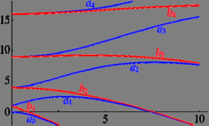
Figure 32 shows the characteristic curves of this equation. We see that now at small the first energy gap grows much faster than the higher ones: n n. This feature is in accord with the weak-coupling result 1 = 2 U 1, which is valid only in the linear approximation in Un, because for the Mathieu potential, Ul = A( l,+1 + l,–1)/2. Another clearly visible feature is the exponentially fast shrinkage of the allowed energy bands at 2 > (in Fig. 32, on the right from the dashed line), i.e. at E < A. It may be readily explained by our tight-binding approximation result (206): as soon as the eigenenergy drops significantly below the potential maximum U max = A (see Fig. 31a), the quantum states in the adjacent potential wells are connected only by tunneling through relatively high potential barriers separating these wells, so the coupling amplitudes n become exponentially small – see, e.g., Eq. (189).
Fig. 2.32. Characteristic curves of the
Mathieu equation. The dashed line
corresponds to the equality = 2, i.e. E =
band
A U max, separating the regions of under-
gap
barrier tunneling and over-barrier motion.
Adapted
from
Fig.
28.2.1
at
http://dlmf.nist.gov as a contribution by the
US Government (not subject to copyright).
Another simple periodic profile is the Kronig-Penney potential shown in Fig. 31b, which gives relatively simple analytical expressions for the band/gap patterns (though transcendent equations for the characteristic curves). Its advantage over the Dirac comb (226) is a more realistic law of the decrease of the Fourier harmonics Ul at l >> 1, and hence of the energy gaps in the weak-potential limit: U
0
( n)
2 U
, at E ~ E
U .
(2.230)
n
n
0
n
Leaving a detailed analysis of the Kronig-Penney potential for the reader’s exercise, let me conclude this section by addressing the effect of potential modulation on the number of eigenstates in 1D systems of a large but finite length l >> a, k-1. Perhaps surprisingly, the Bloch theorem makes the 69 Note that this definition of is quantitatively different from that for the Dirac comb (226), but in both cases, this parameter is proportional to the amplitude of the potential’s periodic modulation.
70 This equation, first studied in the 1860s by É. Mathieu in the context of a rather practical problem of vibrating elliptical drumheads (!), has many other important applications in physics and engineering, notably including the parametric excitation of oscillations – see, e.g., CM Sec. 5.5.
Chapter 2
Page 55 of 76
QM: Quantum Mechanics
analysis of this problem elementary, for arbitrary U( x). Indeed, let us assume that l is comprised of an integer number of periods a, and its ends are described by similar boundary conditions – both assumptions evidently inconsequential for l >> a. Then, according to Eq. (210), the boundary conditions impose, on the quasimomentum q, exactly the same quantization condition as we had for k for a free 1D
motion. Hence, instead of Eq. (1.93), we can write
l
dN
dq ,
(2.231) 1D number
2
of states
with the corresponding change of the summation rule:
l
f ( q)
f ( q) dk .
(2.232)
q
2
As a result, the density of states in the 1D q-space, dN/ dq = l/2, does not depend on the potential profile at all! Note, however, that the profile does affect the density of states on the energy scale, dN/ dE. As an extreme example, on the bottom and at the top of each energy band we have dE/ dq
0, and hence
dN dN dE l dE .
(2.233)
dE
dq
dq
2
dq
This effect of state concentration at the band/gap edges (which survives in higher spatial dimensionalities as well) has important implications for the operation of several important electronic and optical devices, in particular semiconductor lasers and light-emitting diodes.
2.8. Periodic systems: Particle dynamics
The band structure of the energy spectrum of a particle moving in a periodic potential has profound implications not only for its density of states but also for its dynamics. Indeed, let us consider the simplest case of a wave packet composed of the Bloch functions (210), all belonging to the same (say, n th) energy band. Similarly to Eq. (27) for a free particle, we can describe such a packet as i qx q t
( x, t)
a u ( x) e
dq ,
(2.234)
q q
where the a-periodic functions u( x), defined by Eq. (208), are now indexed to emphasize their dependence on the quasimomentum, and ( q) En( q)/ is the function of q describing the shape of the corresponding energy band – see, e.g., Fig. 26b or Fig. 28. If the packet is narrow in the q-space, i.e. if the width q of the distribution aq is much smaller than all the characteristic q-scales of the dispersion relation ( q), in particular than / a, we may simplify Eq. (234) exactly as it was done in Sec. 2 for a free particle, despite the presence of the periodic factors uq( x) under the integral. In the linear approximation of the Taylor expansion, we get a full analog of Eq. (32), but now with q rather than k, and d
v
,
and v
,
(2.235)
gr
q q
ph
q q
0
0
dq
q
where q 0 is the central point of the quasimomentum’s distribution. Despite the formal similarity with Eqs. (33) for the free particle, this result is much more eventful. For example, as evident from the dispersion relation’s topology (see Figs. 26b, 28), the group velocity vanishes not only at q = 0, but at all Chapter 2
Page 56 of 76
QM: Quantum Mechanics
values of q that are multiples of (/ a), i.e. at the bottom and on the top of each energy band. Even more intriguing, the group velocity’s sign changes periodically with q.
This group velocity alternation leads to fascinating, counter-intuitive phenomena if a particle placed in a periodic potential is the subject of an additional external force F( t). (For an electron, this may be, for example, the force exerted by the applied electric field.) Let the force be relatively weak so that the product Fa (i.e. the scale of the energy increment from the additional force per one lattice period) is much smaller than both relevant energy scales of the dispersion relation E( q) – see Fig. 26b: Fa E
, .
(2.236)
n
n
This strong relation enables us to neglect the force-induced interband transitions, so the wave packet (234) includes the Bloch eigenfunctions belonging to only one (initial) energy band at all times. The time evolution of its center q 0 obeys an extremely simple equation of motion:71
Time
evolution
1
of quasi-
q F( t) .
(2.237)
0
momentum
This equation is physically very transparent: it is essentially the 2nd Newton law for the time evolution of the quasimomentum q under the effect of the additional force F( t) only, excluding the periodic force
– U( x)/ x of the background potential U( x). This is very natural, because as Eq. (210) implies, q is essentially the particle’s momentum k averaged over the potential’s period, and the periodic force effect drops out at such an averaging.
Despite the simplicity of Eq. (237), the results of its solution may be highly nontrivial. First, let us use Eqs. (235) and (237) to find the instant group acceleration of the particle (i.e. the acceleration of its wave packet’s envelope):
dv
gr
d d q
d d q dq
d
q dq
d
0
0
2
( )
1 2
0
0
0
a
F( t) .
(2.238)
gr
2
2
q q 0
dt
dt dq
dq
dq
dt
dq
dt
dq
0
0
0
0
This means that the second derivative of the dispersion relation ( q) (specific for each energy band) plays the role of the effective reciprocal mass of the particle at this particular value of q 0: 2
Effective
mass
m
.
(2.239)
ef
2
2
2
2
d / dq
d E / dq
n
For the particular case of a free particle, for which Eq. (216) is exact, this expression is reduced to the original (and constant) mass m, but generally, the effective mass depends on the wave packet’s momentum. According to Eq. (239), at the bottom of any energy band, m ef is always positive but depends on the strength of the particle’s interaction with the periodic potential. In particular, according to Eq. (206), in the tight-binding limit, the effective mass is very large:
2
E )1
(
m
m
m .
(2.240)
ef q
( / a) n
2 a 2
2
n
n
71 The proof of Eq. (237) is not difficult but is more compact in the bra-ket formalism to be discussed in Chapter 4. This is why I recommend to the reader its proof as an exercise after reading that chapter.
Chapter 2
Page 57 of 76
QM: Quantum Mechanics
On the contrary, in the weak-potential limit, the effective mass is close to m at most points of each energy band, but at the edges of the (narrow) bandgaps, it is much smaller. Indeed, expanding Eq. (224) in the Taylor series near point q = qm, we get
2
2
1 dE
l
~2
~2
E
E
U
q U
q ,
(2.241)
( n)
ave
n
E E
2 U dq
n
2 U
n
q q
n
m
where and q~ are defined by Eq. (225), and hence
2
U
m
U m
n
m .
(2.242)
ef
n
q qm
2
2 E ( n)
The effective mass effects in real atomic crystals may be very significant. For example, the charge carriers in silicon have m ef 0.19 m e in the lowest, normally-empty energy band (traditionally called the conduction band), and m ef 0.98 m e in the adjacent lower, normally-filled valence band. In some semiconducting compounds, the conduction-band mass may be even smaller – down to 0.0145 m e in InSb!
However, the effective mass magnitude is not the most surprising effect. A more fascinating corollary of Eq. (239) is that on the top of each energy band, the effective mass is negative – please revisit Figs. 26b, 28, and 29 again. This means that the particle (or more strictly, its wave packet’s envelope) is accelerated in the direction opposite to the applied force. This is exactly what electronic engineers, working with electrons in semiconductors, call holes, characterizing them by a positive mass
m ef, but compensating this sign change by taking their charge e positive. If the particle stays in close vicinity of the energy band’s top (say, due to frequent scattering effects, typical for the semiconductors used in engineering practice), such double sign flip does not lead to an error in calculations of hole’s dynamics, because the electric field’s force is proportional to the particle’s charge, so the particle’s acceleration a gr is proportional to the charge-to-mass ratio.72
However, in some phenomena such simple representation is unacceptable.73 For example, let us form a narrow wave packet at the bottom of the lowest energy band,74 and then exert on it a constant force F > 0 – say, due to a constant external electric field directed along the x-axis. According to Eq.
(237), this force would lead to linear growth of q 0 in time, so in the quasimomentum space, the packet’s center would slide, with a constant speed, along the q axis – see Fig. 33a. Close to the energy band’s bottom, this motion would correspond to a positive effective mass (possibly, somewhat different than the genuine particle’s mass m), and hence be close to the free particle’s acceleration. However, as soon as q 0 has reached the inflection point where d 2 E 1/ dq 2 = 0, the effective mass, and hence its acceleration (238) change signs to negative, i.e. the packet starts to slow down (in the direct space), while still moving ahead with the same velocity in the quasimomentum space. Finally, at the energy band’s top, the particle stops at a certain x max, while continuing to move forward in the q-space.
72 More discussion of this issue may be found in SM Sec. 6.4.
73 The balance of this section describes effects that are not discussed in most quantum mechanics textbooks.
Though, in my opinion, every educated physicist should be aware of them, some readers may skip them at the first reading, jumping directly to the next Sec. 9.
74 Physical intuition tells us (and the theory of open systems, to be discussed in Chapter 7, confirms) that this may be readily done, for example, by weakly coupling the system to a relatively low-temperature environment, and letting it relax to the lowest possible energy.
Chapter 2
Page 58 of 76
QM: Quantum Mechanics
(a)
E
(b)
E( q)
E ( q)
2
1
x / F
0
1
1
E
1
E 1
E ( q)
1
x 0
0
qa
a
0
x
E / F
max
1
Fig. 2.33. The Bloch oscillations (red lines) and the Landau-Zener tunneling (blue arrows) represented in: (a) the reciprocal space of q, and (b) the direct space. On panel (b), the tilted gray strips show the allowed energy bands, while the bold red lines, the Wannier-Stark ladder’s steps.
Now we have two alternative ways to look at the further time evolution of the wave packet along the quasimomentum’s axis. From the extended zone picture (which is the simplest for this analysis, see Fig. 33a),75 we may say that the particle crosses the 1st Brillouin zone’s boundary and continues to go forward in q-space, i.e. down the lowest energy band. According to Eq. (235), this region (up to the next energy minimum at qa = 2) corresponds to a negative group velocity. After q 0 has reached that minimum, the whole process repeats again – and again, and again.
These are the famous Bloch oscillations – the effect which had been predicted, by the same F.
Bloch, as early as 1929 but evaded experimental observation until the 1980s (see below) due to the strong scattering effects in real solid-state crystals. The time period of the oscillations may be readily found from Eq. (237):
q
2 / a
2
t
,
(2.243)
B