

Quantum Mechanics by Konstantin K. Likharev - HTML preview
Download the book in PDF, ePub, Kindle for a complete version.
at kR ,
1
(3.70)
4 R
which is compatible with Eq. (69) only if f+ = –1/4, i.e. if
1
ikR
G(r, '
r )
e
.
(3.71)
R
4
Plugging this result into Eq. (67a), we get the following formal solution of Eq. (66): Scattering
m
( '
r )
problem:
(r)
U ( '
r )
eikRd 3 r' .
(3.72)
s
formal solution
2
2
R
Note that if the function U(r) is smooth, the singularity in the denominator is integrable (i.e. not dangerous); indeed, the contribution of a sphere with some radius R 0, with the center at point r ’, into this integral scales as
3
R 2
R
d R
R dR
4
4 RdR 2
2
R
0.
(3.73)
R
R
R
0
0
R
So far, our result (72) is exact, but its apparent simplicity is deceiving because the wavefunction
on its right-hand side generally includes not only the incident wave I but also the scattered wave s 30 This formula is sometimes called the Lipmann-Schwinger equation, though more frequently this term is reserved for either its operator form or the resulting equation for the spatial Fourier components of and i.
31 Please notice both the similarity and difference between this Green’s function and the propagator discussed in Sec. 2.1. In both cases, we use the linear superposition principle to solve wave equations, but while Eq. (67) gives the solution of the inhomogeneous equation (66), Eq. (2.44) does that for a homogeneous Schrödinger equation.
In the latter case, the elementary wave sources are the elementary parts of the initial wavefunction, rather than of the equation’s right-hand side as in our current problem.
32 See, e.g., EM Sec. 1.2.
Chapter 3
Page 17 of 64
QM: Quantum Mechanics
– see Eq. (64). The most straightforward, and most common simplification of this problem, called the Born approximation,33 is possible if the scattering potential U(r) is in some sense small. (We will derive the quantitative condition of this smallness in a minute.) Since at U(r) = 0, the scattering wave s has to disappear, at small but non-zero U(r), s has to be much smaller than i . In this case, on the right-hand side of Eq. (73), we may ignore s in comparison with i, getting
m
exp ik
'
i
(r)
r
U ( '
r )
eikRd 3 r' .
(3.74) Born
s
2
i
2
approximation
R
Actually, Eq. (74) gives us even more than we wanted: it evaluates the scattered wave at any point, including those within of the scattering object, while to spell out Eq. (62), we only need to find the wave far from the scatterer, at r . However, before going to that limit, we can use Eq. (74) to find a quantitative criterion of the Born approximation’s validity. For that, let us estimate the magnitude of the right-hand side of this equation for a scatterer of a linear size ~ a, and the potential magnitude’s scale U 0. The results are different in the following two limits:
(i) If ka << 1, then inside the scatterer (i.e., at distances r’ ~ a), both exp{ ikr ’} and the second exponent under the integral in Eq. (74) change little, and a crude but fair estimate of the solution’s magnitude is
m
2
~
U a .
(3.75)
s
2
i
0
2
(ii) In the opposite limit ka >>1, the function under the integral is nearly periodic in one of the spatial directions (that of the incident wave’s propagation), so the net integral accumulates only on distances of the order of the de Broglie wavelength, ~ k–1, and the integral is correspondingly smaller: m
a 2
~
U
.
(3.76)
s
2
i
0
2
ka
These relations allow us to spell out the Born approximation’s condition, s << I , as 2
U
max[ ka, ]
1 .
(3.77)
0
2
ma
In the fraction on the right-hand side of this relation, we may readily recognize the scale of the kinetic (quantum-confinement) energy Ea of the particle inside a potential well of a size of the order of a, so the Born approximation is valid essentially if the potential energy of particle’s interaction with the scatterer is smaller than Ea. Note, however, that the estimate (76) is not valid in some special situations when the effects of scattering accumulate in some direction. This is frequently the case for small angles of scattering by extended objects, when ka >> 1, but ka ≾ 1.
33 Named after M. Born, who was the first to apply this approximation in quantum mechanics. However, the basic idea of this approach had been developed much earlier (in 1881) by Lord Rayleigh in the context of electromagnetic wave scattering – see, e.g., EM Sec. 8.3. Note also that the contents of that section repeat some aspects of our current discussion – perhaps regrettably but unavoidably so, because the Born approximation is a centerpiece of the theory of scattering/diffraction for both the electromagnetic waves and the de Broglie waves.
Hence I felt I had to cover it in this course for the benefit of the readers who skipped the EM part of my series.
Chapter 3
Page 18 of 64
QM: Quantum Mechanics
Now let us proceed to large distances r >> r’ ~ a, and simplify Eq. (74) using an approximation similar to the dipole expansions in electrodynamics.34 Namely, in the denominator’s R, we may ignore r’
in comparison with the much larger r, but the exponents require more care, because even if r’ ~ a << r, the product kr’ ~ ka may still be of the order of 1. As Fig. 9a shows, in the first approximation in r’, we may take
R r '
r r n '
r ,
(3.78)
r
and since the directions of the vectors k and r coincide, i.e. k = kn r, we get ikR
ikr ik '
kR kr k '
r ,
e
i.e.
e e
r .
(3.79)
(a)
(b)
R
'
r
detector
k
q
r
a
0
0
ki
n '
r
r
Fig. 3.9. (a) The long-range expansion of R, and (b) the definitions of q, , and .
With this replacement, Eq. (74) yields
m
i
(r)
eikr U ( '
r ) exp (k k ) r
.
(3.80)
s
i
'
2
i
d 3 r'
2
r
This relation is a particular case of a more general formula35
Scattering
f (k, k )
function:
i
ikr
e
,
(3.81)
s
i
definition
r
where f(k, ki) is called the scattering function.36 The physical sense of this function becomes clear from the calculation of the corresponding probability current density j s. For that, generally, we need to use Eq. (1.47) with the gradient operator having all spherical-coordinate components.37 However, at kr >> 1, the main contribution to s, proportional to k >> 1/ r, is provided by differentiating the factor eikr, which changes in the common direction of vectors r and k, so
n
k
,
at kr 1,
(3.82)
s
r
s
s
r
and Eq. (1.47) yields
34 See, e.g., EM Sec. 8.2.
35 It is easy to prove that this form is an asymptotic form of any solution s of the scattering problem (even that beyond the Born approximation) at sufficiently large distances r >> a, k-1.
36 Note that the function f has the dimension of length, and does not account for the incident wave. This is why sometimes a dimensionless function, S = 1 + 2 ikf, is used instead. This function S is called the scattering matrix, because it may be considered a natural generalization of the 1D matrix S defined by Eq. (2.124), to higher dimensionality.
37 See, e.g., MA Eq. (10.8).
Chapter 3
Page 19 of 64
QM: Quantum Mechanics
2
f k
( , k 2
)
j
i
( )
k .
(3.83)
s
i
2
m
r
Plugging this expression and also Eq. (61) into Eq. (62), for the differential cross-section we get simply d
2
f (k, k ) ,
(3.84)
i
d
while the total cross-section is
f (k, k ) 2 d Ω
,
(3.85)
i
so the scattering function f(k, ki) gives us everything we need – and in fact more because the function also contains information about the phase of the scattered wave.
Comparing Eqs. (80) and (81), we see that in the Born approximation, the scattering function is given by the so-called Born integral
m
i
f (k, k )
U (r) e q r d 3 r ,
(3.86) Born
i
2
2
integral
where, just for the notation simplicity, r ’ was replaced with r, and q is the following scattering vector: q k k ,
(3.87)
i
with the length q = 2 k sin( /2), where is the scattering angle between the vectors k and ki – see Fig.
9b. For the differential cross-section, Eqs. (84) and (86) yield38
2
2
d
m
d/ d:
iq r 3
U (r)
e
d r .
(3.88) Born
2
d
2
approximation
This is the basic result of this section; it may be further simplified for spherically symmetric scatterers, with
U (r) U ( r).
(3.89)
In this case, it is convenient to represent the exponent in the Born integral as exp{- iqr cos}, where is the angle between the vectors k (i.e. the direction n r toward the detector) and q (rather than the incident wave vector ki!) – see Fig. 9b. Now, for a fixed q, we can take this vector’s direction for the polar axis of a spherical coordinate system, and reduce Eq. (86) to a 1D integral:
2
m
f (k, k )
r drU ( r) d
sin d exp{ iqr' cos }
i
2
2
2 0
0
0
m
qr
m
2
2sin
2
r drU ( r) 2
U ( r)sin( qr) rdr.
(3.90)
2 2
2
qr
q
0
0
38 Note that according to Eq. (88), in the Born approximation, the scattering intensity does not depend on the sign of the potential U, and also that scattering in a certain direction is completely determined by a specific Fourier component of the function U(r), namely by its harmonic with the wave vector equal to the scattering vector q.
Chapter 3
Page 20 of 64
QM: Quantum Mechanics
As a simple example, let us use the Born approximation to analyze scattering on the following spherically symmetric potential:
2
Ur
r
U exp
.
(3.91)
0
2
2 a
In this particular case, it is better to avoid the temptation to exploit the spherical symmetry by using Eq.
(90), and instead, use the general Eq. (88) because it may be represented as a product of three similar Cartesian factors:
mU
x 2
f (k, k )
0 I I I ,
with I exp
,
(3.92)
i
2
x y z
x
iq x
2
x
dx
2
2 a
and similar integrals for Iy and Iz. From Chapter 2, we already know that the Gaussian integrals like Ix may be readily worked out by complementing the exponent to the full square, in our current case giving
I
x
2
2
q a
2 1/ 2 a exp
x
so
etc.;
,
:
2
(3.93)
2
2
2
2 2
d
mU
mU a
0
I I I
2 2
0
q a
a
e
.
d
2 2 x y z
2
Now, the total cross-section is an integral of d/ d over all directions of the vector k. Since in our case the scattering intensity does not depend on the azimuthal angle , the only nontrivial integration is over the scattering angle (see Fig. 9b again):
2
2
2
d
d
mU a
d 2
sin d 4 2 2
0
π a
exp
2 k sin
2
a sin
d
2
d
d
2
0
0
(3.94)
2
2
2
2
2
2 2
mU a
π mU a
k a
4 2 2
0
π a
exp 2 2 2
k a 1 cos
2
d 1
( cos )
0
1
4
e
.
2
2
2
k
0
Let us analyze these results. In the low-energy limit, ka << 1 (and hence qa << 1 for any scattering angle), the scattered wave is virtually isotropic: d/ d const – a very typical feature of a scalar-wave scattering39 by small objects, in any approximation. Note that according to Eq. (77), the Born expression for , following from Eq. (94) in this limit,
2
2
mU a
8 2 2
0
a
,
(3.95)
2
is only valid if is much smaller than the scale a 2 of the physical cross-section of the scatterer. In the opposite, high-energy limit ka >>1, the scattering is dominated by small angles q/ k ~ 1/ ka ~ / a: 39 Note that this is only true for scalar (e.g., the de Broglie) waves but not the vector ones, in particular, the electromagnetic waves where the intensity of the dipole radiation, and hence the scattering by small objects vanishes in the direction of the incident field’s polarization – see, e.g., EM Eqs. (8.26) and (8.139).
Chapter 3
Page 21 of 64
QM: Quantum Mechanics
2
2
d
mU a
2
0
2 a
2 2 2
exp k a
.
(3.96)
2
d
This is, again, very typical for diffraction. Note, however, that due to the smooth character of the Gaussian potential (91), the diffraction pattern (98) exhibits no oscillations of d/ d as a function of the diffraction angle .
Such oscillations naturally appear for scatterers with sharp borders. Indeed, let us consider a uniform spherical scatterer described by the potential
U , for r R
,
U (r) 0
(3.97)
,
0
otherwise.
In this case, integration by parts of Eq. (90) readily yields
2
2 mU
d
2 mU
0
f (k, k )
qR cos qR sin qR ,
so
qR cos qR sin qR . (3.98)
i
0
2
2
3
2 3
q
d
q
According to this result, the scattered wave’s intensity drops very fast with q, so one needs a semi-log plot (such as that used in Fig. 10) to reveal small diffraction fringes,40 with the n th destructive interference (zero-intensity) point tending to qR = ( n + ½) at n . Since, as Fig. 9b shows, q may only change from 0 to 2 k, these intensity minima are only observable at sufficiently large values of the parameter kR when they correspond to real values of the scattering angle . (At kR >> 1, approximately kR/ of these minima, i.e. “dark rings” of low scattering probability, are observable.) On the contrary, at kR << 1 all allowed values of qR are much smaller than 1, so in this limit, the differential cross-section does not depend on qR, i.e. the scattering by the sphere (as by any object in this limit) is isotropic.
0.1
1
d
0.01
u 2 d
0
g
1 1
0 3
Fig. 3.10. The differential cross-section of
the Born scattering of a particle by a
“hard”
(sharp-border)
sphere
(97),
1 1
0 4
normalized to its geometric cross-section
g R 2 and the square of the potential’s
1 1
0 5
magnitude parameter u
0 U 0/(2/2 mR 2), as
a function of the normalized magnitude of
1 1
0 6
the scattering vector q.
0
1
2
3
4
5
qR /
This example shows that in quantum mechanics, the notions of particle scattering and diffraction are essentially inseparable.
40 Their physics is very similar to that of the Fraunhofer diffraction on a 1D scatterer – see, e.g., EM Sec. 8.4.
Chapter 3
Page 22 of 64
QM: Quantum Mechanics
The Born approximation, while being very simple and used more than any other scattering theory, is not without shortcomings. For example, it is not too difficult (and hence is left for the reader’s exercise) to prove the so-called optical theorem, valid for an arbitrary scatterer: Optical
k
Im f k , k
.
(3.99)
theorem
i
i
4
However, Eq. (86) shows that in the Born approximation, the function f is purely real at q = 0 (i.e. for k
= ki), and hence cannot satisfy the optical theorem. Even more evidently, it cannot describe such a simple effect as a dark shadow ( 0) cast by a virtually opaque object (say, with U >> E). There are several ways to improve the Born approximation, while still keeping its general idea of an approximate treatment of U.
(i) Instead of the main assumption s U 0, we may use a complete perturbation series:
...
(3.100)
s
1
2
with
n
n U 0 , and find successive approximations n one by one. In the 1st approximation, we return to the Born formula, but already the 2nd approximation yields
k
Im f k , k
,
(3.101)
2 i
i
1
4
where 1 is the total cross-section calculated in the 1st approximation, so the optical theorem (99) is
“almost satisfied”.41
(ii) As was mentioned above, the Born approximation does not work very well for the objects stretched along the direction (say, x) of the initial wave vector ki. This deficiency may be corrected by the so-called eikonal 42 approximation, which replaces the plane-wave representation (60) of the incident wave with a WKB-like exponent, though still in the 1st approximation in U 0: x
x
1/ 2
m E U '
r
exp ik r
ikx
i k ' r dx'
i
dx'
i
exp
2
( )
exp
( )
exp
0
0
(3.102)
x
m
exp i kx
U ( '
r )
dx' .
2
k
0
The results of this approach satisfy the optical theorem (99) already in the 1st approximation.
Another way toward quantitative results in the theory of scattering, beyond the Born approximation, may be pursued for spherically symmetric potentials (89); I will discuss it in Sec. 8, after a general discussion of particle motion in such potentials in Sec. 7.
3.4. Energy bands in higher dimensions
In Sec. 2.7, we have discussed the 1D band theory for potential profiles U( x) that obey the periodicity condition (2.192). For what follows, let us notice that the condition may be rewritten as 41 An even simpler way to satisfy the theorem (even in the Born approximation) is to change the definition of the function f(k, ki) so that for forward scattering (k = ki), it includes the incident de Broglie wave as well.
42 From the Greek word , meaning “image”. In our current context, this term is purely historic.
Chapter 3
Page 23 of 64


Essential Graduate Physics
QM: Quantum Mechanics
U ( x X ) U ( x) ,
(3.103)
where X = a, with being an arbitrary integer. One may say that the set of points X forms a periodic 1D lattice in the direct (r-) space. We have also seen that each Bloch state (i.e., each eigenstate of the Schrödinger equation for such periodic potential) is characterized by the quasimomentum q, and its energy does not change if q is changed by a multiple of 2/ a. Hence if we form, in the reciprocal (q-) space, a 1D lattice of points Q = lb, with b 2/ a and integer l, any two points from these two mutually reciprocal lattices satisfy the following rule:
2
exp iQX exp
2
il
a il
e
1,
(3.104)
a
because the product of any two integers l and is also an integer.
In this form, the results of Sec. 2.7 may be readily generalized to d-dimensional periodic potentials whose translational symmetry obeys the following natural generalization of Eq. (103): U (r R) U (r) ,
(3.105)
where the points R, which may be numbered by d integers j, form the so-called Bravais lattice:43
d
R a ,
(3.106) Bravais
j
j
lattice
j1
with d primitive vectors a j. The simplest example of a 3D Bravais lattice is given by the simple cubic lattice (Fig. 11a), which may be described by a system of mutually perpendicular primitive vectors a j of equal length. However, not in any lattice these vectors are perpendicular; for example, Figs. 11b and 11c show possible sets of the primitive vectors describing, respectively, the face-centered cubic (fcc) lattice and the body-centered cubic (bcc) lattice. In 3D, the science of crystallography based on group theory distinguishes, by their symmetry properties, 14 different Bravais lattices, which may be grouped into 7
distinct lattice systems.44
(a)
(b)
(c)
a
a
3
3
a1
a
3
a
2
a1
a
a
2
2
a
1
Fig. 3.11. The simplest (and most common) 3D Bravais lattices: (a) simple cubic, (b) face-centered cubic (fcc), and (c) body-centered cubic (bcc), and possible choices of their primitive vector sets (blue arrows).
43 Named after A. Bravais, the crystallographer who introduced this notion in 1850.
44 An exceptionally clear and well-illustrated introduction to the Bravais lattices is given in Chapters 4 and 7 of the famous textbook by N. Ashcroft and N. Mermin, Solid State Physics, Saunders College, 1976.
Chapter 3
Page 24 of 64


Essential Graduate Physics
QM: Quantum Mechanics
Note, however, not all highly symmetric sets of single points form Bravais lattices. As probably the most striking example, the nodes of the very simple 2D honeycomb lattice (Fig. 12a)45 cannot be described by a Bravais lattice – while those of the 2D hexagonal lattice shown in Fig. 12b, can. The most prominent 3D case of such a lattice is the diamond structure (Fig. 12c), which describes, in particular, silicon crystals.46 In cases like these, the band theory is much facilitated by the fact that the Bravais lattices using some point groups called unit cells (or “bases”, or “cells with basis”, or “motifs”) may describe these systems.47 For example, Fig. 12a shows a possible choice of the primitive vectors for the honeycomb lattice, with the unit cell formed by any two adjacent points of the original lattice (say, within the dashed ovals on that panel). Similarly, the diamond lattice may be described as an fcc Bravais lattice with a two-point unit cell – see Fig. 12c.
(a)
(b)
(c)
a
a
1
2
a3
a2
a
a
1
2
a1
Fig. 3 .12. Two important periodic structures that require two-point unit cells for their Bravais lattice representation: (a) 2D honeycomb lattice and (c) 3D diamond lattice, and their primitive vectors. For contrast, panel (b) shows the 2D hexagonal lattice that forms a Bravais lattice with a single-point unit cell.
Now we are ready for the following generalization of the 1D Bloch theorem, given by Eqs.
(2.193) and (2.210), to higher dimensions: any eigenfunction of the Schrödinger equation describing a particle’s motion in the spatially-unlimited periodic potential (105) may be represented either as iq R
r
( R) r
( ) e
,
(3.107)
3D Bloch or as
theorem
(r) u(r) q
i r
e
, with u(r R) u(r),
(3.108)
where the quasimomentum q is again a constant of motion, but now it is a vector. The key notion of the band theory in d dimensions is the reciprocal lattice in the wave vector (q-) space, formed as Reciprocal
d
lattice in
Q l b ,
(3.109)
j
j
q-space
j1
45 This structure describes, for example, the now-famous graphene – isolated monolayer sheets of carbon atoms arranged in a honeycomb lattice with an interatomic distance of 0.142 nm.
46 This diamond structure may be best understood as an overlap of two fcc lattices of side a, mutually shifted by the vector {1, 1, 1} a/4, so the distances between each point of the combined lattice and its 4 nearest neighbors (see the solid gray lines in Fig. 12c) are all equal.
47 A harder case is presented by so-called quasicrystals (whose idea may be traced down to medieval Islamic tilings, but was discovered in natural crystals, by D. Shechtman et al., only in 1984), which obey a high (say, the 5-fold) rotational symmetry, but cannot be described by a Bravais lattice with any finite unit cell. For a popular review of quasicrystals, see, for example, P. Stephens and A. Goldman, Sci. Amer. 264, #4, 24 (1991).
Chapter 3
Page 25 of 64
QM: Quantum Mechanics
with integer lj, and vectors b j selected in such a way that the following natural generalization of Eq.
(104) is valid for any two points of the direct and reciprocal lattices:
Q
i R
e
1.
(3.110)
One way to describe the physical sense of the lattice Q is to say that according to Eqs. (80) and/or (86), it gives the set of the vectors q k – ki for that the interference of the waves scattered by all Bravais lattice points is constructive, and hence strongly enhanced.48 Another way to look at the reciprocal lattice follows from the first formulation of the Bloch theorem, given by Eq. (107): if we add to the quasimomentum q of a particle any vector Q of the reciprocal lattice, the wavefunction does not change. This means, in particular, that all information about the system’s eigenfunctions is contained inside just one elementary cell of the reciprocal space q. Its most frequent choice, called the 1st Brillouin zone, is the set of all points q that are closer to the origin than to any other point of the lattice Q. (Evidently, the 1st Brillouin zone in one dimension, discussed in Sec. 2.7, falls under this definition –
see, e.g., Figs. 2.26 and 2.28.)
It is easy to see that the primitive vectors b j of the reciprocal lattice may be constructed as Reciprocal
a a
a a
a a
2
3
3
1
1
2
b 2
, b 2
, b 2
.
(3.111) lattice:
1
a a a
a a a
a a a
primitive
1 2
2
3
1 2
3
3
1 2
3
vectors
Indeed, from the “operand rotation rule” of the vector algebra49 it is evident that a jb j’ = 2 jj’. Hence, with the account of Eq. (109), the exponent on the left-hand side of Eq. (110) is reduced to eiQ R
exp 2 i l l l
.
(3.112)
1 1
2 2
3 3
Since all lj and all j are integers, the expression in the parentheses is also an integer, so the exponent indeed equals 1, thus satisfying the definition of the reciprocal lattice given by Eq. (110).
As the simplest example, let us return to the simple cubic lattice of a period a (Fig. 11a), oriented in space so that
a an , a an , a an .
(3.113)
1
x
2
y
3
z
According to Eq. (111), its reciprocal lattice is also simple cubic:
2
Q
( l n l n l n ) ,
(3.114)
x
x
y
y
z
z
a
so the 1st Brillouin zone is a cube with the side b = 2/ a.
Almost equally simple calculations show that the reciprocal lattice of fcc is bcc, and vice versa.
Figure 13 shows the resulting 1st Brillouin zone of the fcc lattice.
The notion of the reciprocal lattice makes the multi-dimensional band theory not much more complex than that in 1D, especially for numerical calculations, at least for the single-point Bravais 48 This is why the notion of the Q-lattice is also the main starting point of X-ray diffraction studies of crystals.
Indeed, it allows rewriting the well-known Bragg condition for diffraction peaks in an extremely simple form: k =
ki + Q, where ki and k are the wave vectors of the, respectively, incident and diffracted waves – see, e.g., EM Sec.
8.4 (where it was more convenient for me to use the notation k0 for ki ).
49 See, e.g., MA Eq. (7.6).
Chapter 3
Page 26 of 64

Essential Graduate Physics
QM: Quantum Mechanics
lattices. Indeed, repeating all the steps that have led us to Eq. (2.218), but now with a d-dimensional Fourier expansion of the functions U(r) and u(r), we readily get its generalization:
U u ( E E u
)
l '
,
(3.115)
l l '
l
l
l ' l
where l is now a d-dimensional vector of integer indices lj. The summation in Eq. (115) should be carried over all essential components of this vector (i.e. over all relevant nodes of the reciprocal lattice), so writing a corresponding computer code requires a bit more care than in 1D. However, this is just a homogeneous system of linear equations for coefficients ul, and numerous routines of finding its eigenvalues E are readily available from both public sources and commercial software packages.
qz
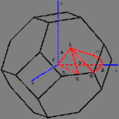
Fig. 3.13. The 1st Brillouin zone of the fcc
q
y
lattice, and the traditional notation of its
main
directions.
Adapted
from
qx
http://en.wikipedia.org/wiki/Band_structure,
as a public domain material.
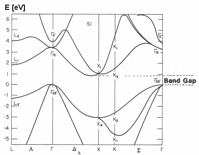
What is indeed more complex than in 1D is the representation (and hence comprehension :-) of the calculated results and experimental data. Typically, the representation is limited to plotting the Bloch state eigenenergy as a function of the vector q’s components along certain special directions in the reciprocal space of quasimomentum (see, e.g., the red lines in Fig. 13), typically on a single panel.
Fig. 14 shows perhaps the most famous (and certainly the most practically important) of such plots, the band structure of electrons in crystalline silicon. The dashed horizontal lines mark the so-called indirect gap of width ~1.12 eV between the lower “valence” (nominally occupied) and the next “conduction”
(nominally unoccupied) energy bands.
Fig. 3.14. The band structure of silicon, plotted along
the special directions shown in Fig. 13. (Adapted from
https://www.tf.uni-kiel.de/matwis/amat/semi_en/.)
Chapter 3
Page 27 of 64
QM: Quantum Mechanics
In order to understand the reason for such complexity, let us see how would we start to calculate such a picture in the weak-potential approximation, for the simplest case of a 2D square lattice – which is a subset of the cubic lattice (106), with 3 = 0. Its 1st Brillouin zone is of course also a square, of the area (2/ a)2 – see the dashed lines in Fig. 15. Let us draw the lines of the constant energy of a free particle ( U = 0) in this zone. Repeating the arguments of Sec. 2.7 (see especially Fig. 2.28 and its discussion), we may conclude that Eq. (2.216) should be now generalized as follows, 2
2
2
2
2
k
2 l
2 l
x
y
E
q
,
(3.116)
x
q
2 m
2 m
y
a
a
with all possible integers lx and ly. Considering this result only within the 1st Brillouin zone, we see that as the particle’s energy E grows, the lines of equal energy, for the lowest energy band, evolve as shown in Fig. 15. Just like in 1D, the weak-potential effects are only important at the Brillouin zone boundaries and may be crudely represented as the appearance of narrow energy gaps. However, one can see that the band structure in the q-space is complex enough even without these effects – and becomes even more involved at higher E.
qy
(a)
(b)
(c)
Fig. 3.15. The lines of constant
2
energy E of a free particle, within
the 1st Brillouin zone of a square
a
0
qx
Bravais lattice, for: (a) E/ E
1 0.95,
(b) E/ E 1 1.05; and (c) E/ E 1 2.05,
where E 1 22/2 ma 2.
2 / a
The tight-binding approximation is usually easier to follow. For example, for the same square 2D
lattice, we may repeat the arguments that have led us to Eq. (2.203), to write 50
i a
a
a
a
a
,
(3.117)
0,0
n ,
1 0
,
1 0
0, 1
0, 1
where the indices correspond to the deviations of the integers x and y from an arbitrarily selected minimum of the potential energy – and hence of the wavefunction’s “hump” that is quasi-localized at this minimum. Now, looking for the stationary solution of these equations, that would obey the Bloch theorem (107), instead of Eq. (2.206) we get
iq a
iq a
iq a
iq a
E E E e x e
x
e y e
y
E 2
(3.118)
n
n
n
n
n
n cos q a
cos q a
x
y
.
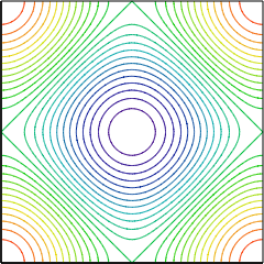
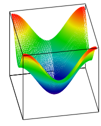
Figure 16 shows this result, within the 1st Brillouin zone, in two forms: as color-coded lines of equal energy, and as a 3D plot. It is evident that the plots of this function along different lines on the q-
plane, for example along one of the axes (say, qx) and along a diagonal of the 1st Brillouin zone (say, with qx = qy) give different curves E( q), qualitatively similar to those of silicon (Fig. 14).
50 Actually, using the same values of n in both directions ( x and y) implies some sort of symmetry of the quasi-localized states. For example, the s-states of axially-symmetric potentials (see the next section) always have such symmetry.
Chapter 3
Page 28 of 64
Essential Graduate Physics
QM: Quantum Mechanics
qy
n
4 n
2
0
q
0
q
x
a
y
Fig. 3.16. The allowed band
energy n E – En for a square
4 n
qx
2D lattice, in the tight-binding
approximation.
2 / a
However, the latter structure is further complicated by the fact that the unit cell of its Bravais lattice contains two atoms – see Fig. 12c and its discussion. In this case, even the tight-binding picture becomes more complex. Indeed, even if the atoms at different positions of the unit cell are similar (as they are, for example, in both graphene and silicon), and hence the potential wells near those points and the corresponding local wavefunctions u(r) are similar as well, the Bloch theorem (which only pertains to Bravais lattices!) does not forbid them from having different complex probability amplitudes a( t) whose time evolution should be described by a specific differential equation.
As the simplest example, to describe the honeycomb lattice shown in Fig. 12a, we have to prescribe different probability amplitudes to the “top” and “bottom” points of its unit cell – say, and , correspondingly. Since each of these points is surrounded (and hence weakly interacts) with three neighbors of the opposite type, instead of Eq. (117) we have to write two equations: 3
3
i
i
,
(3.119)
n
,
j
n
j'
j1
j' 1
where each summation is over three nearest-neighbor points. (In these two sums, I am using different summation indices just to emphasize that these directions are different for the “top” and “bottom” points of the unit cell – see Fig. 12a.) Now using the Bloch theorem (107) in the form similar to Eq. (2.205), we get two coupled systems of linear algebraic equations:
3
3
i
q r
i '
q r
E E
e
E E
e
(3.120)
n
n
j ,
n n j' ,
j 1
j' 1
where r j and r ’j’ are the nearest-neighbor positions, as seen from the top and bottom points, respectively.
Writing the condition of consistency of this system of homogeneous linear equations, we get two equal and opposite values for energy correction for each value of q:
3
'
1/ 2
iq r
j
r j'
E E ,
where
.
(3.121)
e
n
n
j, j'1
According to Eq. (120), these two energy bands correspond to the phase shifts (on the top of the regular Bloch shift qr) of either 0 or between the adjacent quasi-localized wavefunctions u(r ).
Chapter 3
Page 29 of 64
QM: Quantum Mechanics
The most interesting corollary of such energy symmetry, augmented by the honeycomb lattice’s symmetry, is that for certain values qD of the vector q (that turn out to be in each of six corners of the honeycomb-shaped 1st Brillouin zone), the double sum vanishes, i.e. the two band surfaces E(q) touch each other. As a result, in the vicinities of these so-called Dirac points,51 the dispersion relation is linear:
~
~
E
E v q ,
where q q q ,
(3.122)
q q
n
n
D
D
with vn n being a constant with the dimension of velocity – for graphene, close to 106 m/s. Such a linear dispersion relation ensures several interesting transport properties of graphene, in particular of the quantum Hall effect in it – as was already mentioned in Sec. 2. For their more detailed discussion, I have to refer the reader to special literature.52
3.5. Axially symmetric systems
I cannot conclude this chapter (and hence our review of wave mechanics) without addressing the exact solutions of the stationary Schrödinger equation53 possible in the cases of highly symmetric functions U(r). Such solutions are very important, in particular, for atomic and nuclear physics, and will be used in the later chapters of this course.
In some rare cases, such symmetries may be exploited by the separation of variables in Cartesian coordinates. The most famous (and rather important) example is the d-dimensional isotropic harmonic oscillator – a particle moving inside the potential well
2
d
m
U
0 r 2 .
(3.123)
j
2
j1
Separating the variables exactly as we did in Sec. 1.7 for the rectangular hard-wall box (1.77), for each degree of freedom we get the Schrödinger equation (2.261) of a 1D oscillator, whose eigenfunctions are 51 This term is based on a (rather indirect) analogy with the Dirac theory of relativistic quantum mechanics, to be discussed in Chapter 9 below.
52 See, e.g., the reviews by A. Castro Neto et al., Rev. Mod. Phys. 81, 109 (2009) and by X. Lu et al., Appl. Phys.
Rev. 4, 021306 (2017). Note that the transport properties of graphene are determined by coupling of 2 pz- states of its carbon atom electrons (see Secs. 6 and 7 below), whose wavefunctions are proportional to exp{ i} rather than are axially symmetric as implied by Eqs. (120). However, due to the lattice symmetry, this fact does not affect the above dispersion relation E(q).
53 This is my best chance to mention, in passing, that the eigenfunctions n(r) of any such problem do not feature the instabilities typical for the deterministic chaos effects of classical mechanics – see, e.g., CM Chapter 9. (This is why the term quantum mechanics of classically chaotic systems is preferable to the occasionally used term
“quantum chaos”.) It is curious that at the initial stages of the time evolution of the wavefunctions of such systems, their certain correlation functions still grow exponentially, reminding the Lyapunov exponents of their classical chaotic dynamics. This growth stops at the so-called Ehrenfest times t E ~ -1ln( S/), where S is the action scale of the problem – see, e.g., I. Aleiner and A. Larkin, Phys. Rev. E 55, R1243 (1997). In a stationary quantum state, the most essential trace of the classical chaos in a system is the unusual statistics of its eigenvalues, in particular of the energy spectra. We will have a chance for a brief look at such statistics in Chapter 5, but unfortunately, I will not have time/space to discuss this field in much detail. Perhaps the best available book for further reading is the monograph by M. Gutzwiller, Chaos in Classical and Quantum Mechanics, Springer, 1991.
Chapter 3
Page 30 of 64

Essential Graduate Physics
QM: Quantum Mechanics
given by Eq. (2.284), and the energy spectrum is described by Eq. (2.162). As a result, the total energy spectrum may be indexed by a vector n = { n 1, n 2,…, nd} of d independent integer quantum numbers nj:
d
d
E
,
(3.124)
n
n
0
j
j1
2
each ranging from 0 to . Note that every energy level of this system, with the only exception of its ground state,
d
1
d
1
( )
exp
,
(3.125)
g
r
r 2
0
j
d / 4
d / 2
2 j
j1
x
2
0
x 0 j1
is degenerate: several different wavefunctions, each with its own different set of the quantum numbers nj, but the same value of their sum, have the same energy.
However, the harmonic oscillator problem is an exception: for other axially and spherically symmetric problems, the solution is made much easier by using the appropriate curvilinear coordinates.
Let us start with the simplest axially symmetric problem: the so-called planar rotor (or “rotator”), i.e. a particle of mass m,54 constrained to move along a plane circle of radius R (Fig. 17).55
n m
R
l
R
0
Fig. 3.17. A planar rigid rotor.
The classical state of such planar rotor may be described by just one coordinate, say, the angular displacement (or equivalently, the arc displacement l R) from some reference direction, with the energy (and the Hamiltonian function) H = p 2/2m, where p mv = mn( dl/ dt), n being the unit vector in the azimuthal direction – see Fig. 17. This function is similar to that of a free 1D particle (with the replacement x l R), and hence the rotor’s quantum properties may be described by a similar Hamiltonian operator:
p ˆ2
ˆ
H
,
p
with ˆ in
i n
,
(3.126)
2m
l
R
whose eigenfunctions have a similar structure:
ikl
ikR
Ce
Ce
.
(3.127)
54 From this point on (until the chapter’s end), I will use this exotic font for the particle’s mass, to avoid any chance of its confusion with the impending “magnetic” quantum number m, traditionally used in axially-symmetric problems.
55 This is a reasonable model for the confinement of light atoms, notably hydrogen, in some organic compounds, but I am addressing this system mostly as the basis for the forthcoming, more complex problems.
Chapter 3
Page 31 of 64
QM: Quantum Mechanics
The “only” new feature is that in the rotor, all observables should be 2-periodic functions of the angle . Hence, as we have already discussed in the context of the magnetic flux quantization (see Fig. 4
and its discussion), as the particle makes one turn around the central point 0, its wavefunction’s phase kR may only change by 2 m, with an arbitrary integer m (ranging from – to +): 2 im
(
2 ) ( ) e
.
(3.128)
m
m
With the eigenfunctions (127), this periodicity condition immediately gives 2 kR = 2 m. Thus, the wave number k can take only quantized values km = m/ R, so the eigenfunctions should be indexed by this magnetic quantum number m:
l
C exp im
C exp
,
(3.129) Planar rotor:
m
m
m
im
R
eigenfunctions
and the energy spectrum is discrete56:
2
2
2
2
2
p
k
m
m
E
m
.
(3.130) Planar rotor:
m
2
2m
2m
2m R
eigenenergies
This simple model allows exact analysis of an external magnetic field’s effect on a confined motion of an electrically charged particle. Indeed, in the simplest case when this field is axially symmetric (or just uniform) and directed normally to the rotor’s plane, it does not violate the axial symmetry of the system. According to Eq. (26), in this case, we have to generalize Eq. (126) as 2
2
1
1
ˆ
H
in
A
q
i n
A
q
.
(3.131)
2m
l
2
m
R
Here, in contrast to the Cartesian gauge choice (44), which was so instrumental for the solution of the Landau level problem, it is beneficial to take the vector potential in the axially symmetric form A =
A()n, where { x, y} is the 2D radius vector, with the magnitude = ( x 2 + y 2)1/2. Using the well-known expression for the curl operator in the cylindrical coordinates,57 we can readily check that the requirement A = Bn z, with B = const, is satisfied by the following function (which was already mentioned in Sec. 2):
B
A n
.
(3.132)
2
For the planar rotor, ρ = R = const, so the stationary Schrödinger equation becomes 1
2
B R
i
q
E .
(3.133)
2
m
R
2
m
n
m
A little bit surprisingly, this equation is still satisfied with the eigenfunctions (127)! Moreover, since the periodicity condition (128) is also unaffected by the applied magnetic field, we return to the periodic eigenfunctions (129), independent of B. However, the field does affect the system’s eigenenergies:
56 Note that Em does not include the radial confinement energy. (See Sec. 2.1 and the solution of Problem 2.1.) 57 See, e.g., MA Eq. (10.5).
Chapter 3
Page 32 of 64
QM: Quantum Mechanics
2
2
2
2
Planar rotor:
1 1
R
B
1 m
R
B
Φ
magnetic
E
i
q
,
(3.134)
m
m
q
m
2
field’s effect
2
m
m
R
2
2m R
2
2
R
m
Φ
' 0
where R 2B is the magnetic flux through the area limited by the particle’s trajectory, and 0 ’
2/ q is the “normal” magnetic flux quantum we have already met in the AB effect’s context – see Eq.
(34) and its discussion. The field also changes the circular electric current of the particle for each m:
*
iqR B
2
I q
c.c.
.
(3.135)
m
m
m
q
Cm m
2 i m R
2
m R
' 0
Normalizing the wavefunction (129) to have Wm = 1, we get Cm 2 = 1/2 R, so Eq. (135) becomes
Φ
q
I m
I ,
with I
.
(3.136)
m
Φ
0
0
'
2
2
m R
0
The functions Em() and Im () are shown in Fig. 18. Note that since 0 ’ 1/ q, for any sign of the particle’s charge q, dIm/ d < 0. It is easy to verify that this means that the current is diamagnetic for any sign of q:58 the field-induced current flows in such a direction that its own magnetic field tries to compensate for the external magnetic flux applied to the loop. This result may be interpreted as a different manifestation of the AB effect.59 In contrast to the interference experiment that was discussed in Sec. 1, in the situation shown in Fig. 17 the particle is not absorbed by the detector but travels around the ring continuously. As a result, its wavefunction is “rigid”: due to the periodicity condition (128), the quantum number m is discrete, and the applied magnetic field cannot change the wavefunction gradually. In this sense, the system is similar to a superconducting loop – see Fig. 4 and its discussion.
The difference between these systems is two-fold:
Em
m 1
m 0
m
1
0
1
/ ' 0
I
m
Fig. 3.18. The magnetic field’s effect on a
charged planar rotor. Dashed arrows show
possible inelastic transitions between
metastable and ground states, due to weak
0
1
/ ' 0 interaction with the environment, as the
m 1
m 0
m 1
external magnetic field is slowly increased.
58 This effect, whose qualitative features remain the same for all 2D or 3D localized states (see Chapter 6 below), is frequently referred to as orbital diamagnetism. In magnetic materials consisting of particles with uncompensated spins, this effect competes with an opposite effect, spin paramagnetism – see, e.g., EM Sec. 5.5.
59 It is straightforward to check that the final forms of Eqs. (134)-(136) remain valid even if the magnetic field is localized well inside the rotor’s circumference so its lines do not touch the particle’s trajectory.
Chapter 3
Page 33 of 64
QM: Quantum Mechanics
(i) For a single charged particle, in macroscopic systems with practicable values of q, R, and m, the scale I 0 of the induced current is very small. For example, for m = m e, q = – e, and R = 1 m, Eq.
(136) yields I 0 3 pA.60 With the ring’s inductance L of the order of 0 R,61 the contribution I = L I ~
0 RI 0 ~ 10–24 Wb of such a small current to the net magnetic flux is negligible in comparison with 0 ’
~ 10–15 Wb, so the wavefunction quantization does not lead to the constancy of the total magnetic flux.
(ii) As soon as the magnetic field raises the eigenstate energy Em above that of another eigenstate Em’, the former state becomes metastable, and a weak interaction of the system with its environment (which is neglected in our simple model, but will be discussed in Chapter 7) may induce a quantum transition of the system to the lower-energy state, thus reducing the diamagnetic current’s magnitude –
see the dashed lines in Fig. 18. The flux quantization in superconductors is much more robust to such perturbations.62
Now let us return, once again, to the key Eq. (129), and see what it gives for one more important observable, the particle’s angular momentum
L r p ,
(3.137)
In this particular geometry, the vector L has just one component, normal to the rotor plane: L Rp .
(3.138)
z
In classical mechanics, the rotor’s Lz should be conserved (due to the absence of an external torque), but it may take arbitrary values. In quantum mechanics, the situation changes: with p = k, our result km =
m/ R for the m th eigenstate may be rewritten as
Angular
( L ) R k m .
(3.139) momentum
z m
m
quantization
Thus, the angular momentum is quantized: it may be only a multiple of the Planck constant –
confirming the N. Bohr’s guess – see Eq. (1.8). As we will see in Chapter 5, this result is very general (though it may be modified by spin effects), and the wavefunctions (129) may be interpreted as eigenfunctions of the angular momentum operator.
Let us see whether this quantization persists in more general but still axial-symmetric systems.
To implement the planar rotor in our 3D world, we needed to provide rigid confinement of the particle both in the motion plane and along the 2D radius . Let us consider a more general situation when only the former confinement is strict, i.e. the case when a 2D particle moves in an arbitrary axially symmetric potential
U (ρ) U () .
(3.140)
60 Such weak persistent, macroscopic diamagnetic currents in non-superconducting systems have been experimentally observed by measuring the weak magnetic field induced by the currents, in systems of a large number (~107) of similar conducting rings – see L. Lévy et al., Phys. Rev. Lett. 64, 2074 (1990). Due to the dephasing effects of electron scattering by phonons and other electrons (unaccounted for in our simple theory), the effect’s observation required submicron rings and millikelvin temperatures.
61 See, e.g., EM Sec. 5.3.
62 Interrupting a superconducting ring with a weak link (Josephson junction), i.e. forming a SQUID, we may get a switching behavior similar to that shown with dashed arrows in Fig. 18 – see, e.g., EM Sec. 6.5.
Chapter 3
Page 34 of 64
QM: Quantum Mechanics
Using the well-known expression for the 2D Laplace operator in polar coordinates,63 we may represent the 2D stationary Schrödinger equation in the form
2
1
1 2
.
(3.141)
2
2
U (
)
E
2m
Separating the radial and angular variables as64
R () F () ,
(3.142)
we get, after the division of all terms by and their multiplication by ρ 2, the following equation: 2
d dR 1 d 2
F
U
2
2
() E .
(3.143)
2m R d d F d 2
The fraction ( d 2 F/ d2)/ F should be a constant (because all other terms of the equation may be functions only of ρ), so for the function F() we get an ordinary differential equation, 2
d
F
2
F 0,
(3.144)
2
d
where 2 is the variable separation constant. The fundamental solutions of Eq. (144) are evidently F
exp{ i}. Now requiring, as we did for the planar rotor, the 2 periodicity of any observable, i.e.
2 im
F
(
2 ) F ( ) e
,
(3.145)
where m is an integer, we see that the constant has to be equal to m. Thus we get, for the angular factor, the same result as for the full wavefunction of the planar rotor – cf. Eq. (129):
C eim
F
,
with m ,
0 ,
1 ,...
2
(3.146)
m
m
Plugging the resulting relation ( d 2 F/ d2)/ F = – m 2 back into Eq. (143), we may rewrite it as 2
1 d dR m 2
.
(3.147)
2 U (
) E
2m R d d
The physical interpretation of this equation is that the full energy is a sum,
E E E ,
(3.148)
of the radial-motion part
2
1 d dR
E
()
U
.
(3.149)
2m
d
d
and the angular-motion part
63 See, e.g., MA Eq. (10.3) with / z = 0.
64 At this stage, I do not want to mark the particular solution (eigenfunction) and corresponding eigenenergy E
with any single index, because based on our experience in Sec. 1.7, we already may expect that in a 2D problem, the role of this index will be played by two integers – two quantum numbers.
Chapter 3
Page 35 of 64
QM: Quantum Mechanics
2
2
m
E
.
(3.150)
2
2m
Now let us recall that a similar separation exists in classical mechanics, because the total energy of either 2D or 3D particle moving in a central field may be represented as 65
m 2
E
v U () m 2
2
2
U() E E ,
(3.151)
2
2
2
2
2
p
p
L
m 2 2
with E
U (),
and E
z
.
(3.152)
2
2m
2
2m
2
m
The comparison of the latter relation with Eqs. (139) and (150) gives us grounds to expect that the quantization rule Lz = m may be valid not only for this 2D problem but in 3D cases as well. In Sec. 5.6
below, we will see that this is indeed the case.
Returning to Eq. (147), with our 1D wave mechanics experience we may expect that at any fixed m, this ordinary, linear, second-order differential equation should have (for a motion confined to a certain final region of its argument ρ) a discrete energy spectrum described by another integer quantum number – say, n. This means that the eigenfunctions (142) and corresponding eigenenergies (148) and R( ρ) should be indexed by two quantum numbers, m and n. So, the variable separation is not as “clean”
as it was for the rectangular potential well. Normalizing the angular function F to the full circle, =
2, we may rewrite Eq. (142) as
1
R () F
im
( )
R ( )
.
(3.153)
m, n
m,n
m
2
e
1/2 m,n
A good (and important) example of an analytically solvable problem of this type is a 2D particle whose motion is rigidly confined to a disk of radius R, but otherwise free:
,
0
0
for R,
U ()
(3.154)
, for R .
In this case, the solutions Rm,n() of Eq. (147) are proportional to the first Bessel functions Jm( knρ), ща
еру ашкые лштв66 with the spectrum of possible values kn following from the boundary condition Rm,n( R) = 0. Let me leave a detailed analysis of this problem for the reader’s exercise.
3.6. Spherically symmetric systems: Brute force approach
Now let us proceed to the mathematically more involved, but practically even more important case of the 3D motion in a spherically symmetric potential
U (r) U ( r).
(3.155)
65 See, e.g., CM Sec. 3.5.
66 A summary of the main properties of these functions, including the most important plots and a useful table of values, may be found in EM Sec. 2.7.
Chapter 3
Page 36 of 64
QM: Quantum Mechanics
Let us start, again, with solving the eigenproblem for a rotor – now a spherical rotor, i.e. a particle confined to move on the spherical surface of radius R. The classical rotor’s position on the surface is completely described by two coordinates – say, the polar angle and the azimuthal angle .
Its kinetic energy is limited to the angular motion, so for the quantum-mechanical description, in the Laplace operator expressed in spherical coordinates67 we may keep only those parts, with fixed r = R.
Because of this, the stationary Schrödinger equation becomes
2
1
1
2
sin
E .
(3.156)
2
2
2
2 R
m
sin
sin
(Again, we will attach indices to and E in a minute.) With the natural variable separation,
( ) F () ,
(3.157)
Eq. (156), with all terms multiplied by sin2/ F, yields
2
sin
2
d
d 1 d F
sin
2
E sin .
(3.158)
2
2 R
m
d
d
2
F d
Just as in Eq. (143), the fraction ( d 2 F/ dx 2)/ F may be a function of only and hence has to be constant, giving Eq. (144) for it. So, with the same periodicity condition (145), the azimuthal functions are expressed by (146) again; in the normalized form,
1
F
im
( )
e
.
(3.159)
m
2 1/ 2
With this, the fraction ( d 2 F/ d2)/ F in Eq. (158) equals (- m 2), and after the multiplication of all terms of that equation by /sin2, it is reduced to the following ordinary linear differential equation for the polar eigenfunctions ():
2
2
1
d
d
m
sin
,
with
E
.
(3.160)
2
2
sin d
d sin
2 R
m
It is common to recast it into an equation for a new function P() (), with cos : 2
d
dP
m
1
2
l l
1
P 0
,
(3.161)
d
d
1
2
where a new notation for the normalized energy is introduced: l( l+1) . The motivation for such notation is that, according to the mathematical analysis of Eq. (161) with integer m,68 it has physically suitable solutions, with P being an either odd or even function of , only if l (called the orbital quantum number) is an integer: l = 0, 1, 2,…, and only it is not smaller than m , i.e. if
l m l .
(3.162)
67 See, e.g., MA Eq. (10.9).
68 This analysis was first carried out by A.-M. Legendre (1752-1833). Just as a historic note: besides many original mathematical achievements, Dr. Legendre had authored a famous textbook, Éléments de Géométrie, which dominated teaching geometry through the 19th century.
Chapter 3
Page 37 of 64
QM: Quantum Mechanics
This fact immediately gives the following spectrum of the spherical rotor’s angular69 energy E – and, as we will see later, that of any spherically symmetric system:
2 l l
1
Angular
E
,
(3.163) energy
l
2
2
R
m
spectrum
so the only effect of the magnetic quantum number m here is imposing the restriction (162) on the non-negative orbital quantum number l. This means, in particular, that each energy level (163) corresponds to (2 l + 1) different values of m, i.e. is (2 l + 1)–degenerate.
To understand the nature of this degeneracy, we need to explore the corresponding eigenfunctions of Eq. (161). They are naturally numbered by two integers, m and l, and are called the a ssociated Legendre functions P m
l . (Note that here m is an upper index, not a power!) For the particular, simplest case m = 0, these functions are the so-called Legendre polynomials P
0
l() P l (), which may
be defined as the solutions of the following Legendre equation, resulting from Eq. (161) at m = 0: d
d
Legendre
1
2
P l l
1 P 0
,
(3.164)
d
d
equation
and may be calculated explicitly from the following Rodrigues formula:70
1 d l
P ( )
( 2
)
1 l , l ,
0 ,
1 ,...
2 .
(3.165) Legendre
l
2 l !
l d l
polynomials
Using this formula, it is easy to spell out a few lowest Legendre polynomials:
1
2
1
P ( ) ,
1
P ( ) , P ( )
P
,
(3.166)
0
1
2
3
1, ( )
3
5 3 3 ,...
2
2
though such explicit expressions become bulkier and bulkier as l is increased. As these expressions (and Fig. 19) show, as the argument is increased, all these functions end up at the same point, Pl(+1) = + 1, while starting at either at the same point or at the opposite point: Pl(–1) = (–1) l.
1
0.5
P ( ) 0
l
4
3
0.5
2
l
1
Fig. 3.19. A few lowest Legendre polynomials.
1
1
0.5
0
0.5
1
cos
69 This qualification is important because this E does not include the energy of radial confinement – see Sec. 2.1.
70 This wonderful formula may be readily proved by plugging it into Eq. (164), but was not so easy to discover!
This was done (independently) by B. O. Rodrigues in 1816, J. Ivory in 1824, and C. Jacobi in 1827.
Chapter 3
Page 38 of 64
QM: Quantum Mechanics
On the way between these two endpoints, the l th polynomial crosses the horizontal axis exactly l times, i.e. Eq. (164) has exactly l roots. (In this behavior, we may readily recognize the “standing wave”
pattern typical for all 1D eigenproblems – cf. Figs. 1.8 and 2.35, as well as the discussion of the Sturm oscillation theorem at the end of Sec. 2.9.) It is also easy to use the Rodrigues formula (165) and the integration by parts to show that on the segment –1 +1, th polynomials form a full orthogonal set of functions, with the following normalization rule:
1
2
P ( ) P ( ) d
.
(3.167)
l
l '
ll '
2 l 1
1
For m > 0, the associated Legendre functions (now not necessarily polynomials!), may be expressed via the Legendre polynomials (165) using the following formula:71
m
Associated
d
Legendre
m
P ( ) ( )
1 m 1
(
2
) m/2
P ( ) ,
(3.168)
l
functions
m l
d
while the functions with a negative magnetic quantum number may be found as
m
m ( l m)!
P ( ) ( )
1
Pm ( ),
for m 0 .
(3.169)
l
( l m)! l
On the segment –1 +1, the associated Legendre functions with a fixed index m form a full orthogonal set, with the normalization relation
1
m
m
2 ( l m)!
P ( ) P ( ) d
,
(3.170)
l
l '
ll '
2 l 1 ( l m)!
1
which is evidently a generalization of Eq. (167) to arbitrary m.
Since the difference between the angles and is, to a large extent, artificial (due to an arbitrary direction of the polar axis), physicists prefer to use not the functions () m P (cos) and
l
Fm() eim
separately, but normalized products of the type (157), which are called the s pherical harmonics: 1/ 2
Spherical
m
l 2 1 l( m)!
harmonics
m
im
Y
( ,)
P (cos ) e
.
(3.171)
l
4
l
( m
l
)!
The specific front factor in Eq. (171) is chosen in a way to simplify the following two expressions: the relation of the spherical harmonics with opposite signs of the magnetic quantum number:
m
Y
( ,) ( )
1 m Y
,
(3.172)
l
m(,)
l
and the following normalization relation:
m
Y ( , Y
d
,
(3.173)
l
m'
)
( , )
l '
ll ' mm'
4
71 Note that some texts use different choices for the front factor (called the Condon-Shortley phase) in the functions P m
m
l , which do not affect the final results for the spherical harmonics Yl .
Chapter 3
Page 39 of 64
QM: Quantum Mechanics
with the integration over the whole solid angle. The last formula shows that on a spherical surface, the spherical harmonics form an orthonormal set of functions. This set is also full, so any function defined on the surface may be uniquely represented as a linear combination of Y m
l .
Despite the somewhat intimidating character of the formulas given above, they yield quite simple expressions for the lowest spherical harmonics, which are most important for applications: 0
l 0 : Y 1/ 4
,
(3.174)
0
1/2
1
Y
i
e
1
3/8 1/2
sin
,
l 1:
0
Y
(3.175)
1
3/ 4 1/2 cos
,
1
1/ 2
i
Y
e
1
3/8
sin
,
2
Y
i
e
2
15/32 1/2 2 2
sin
,
1
Y
i
e
2
15/8 1/2
sin cos
,
l 2
:
0
Y
(3.176)
2
3/16 1/2 3
( cos2
),
1
1 Y
i
e
2
15/8 1/2 sin cos
,
2
1/ 2
2
2
i
Y
e
2
15/32 sin
.
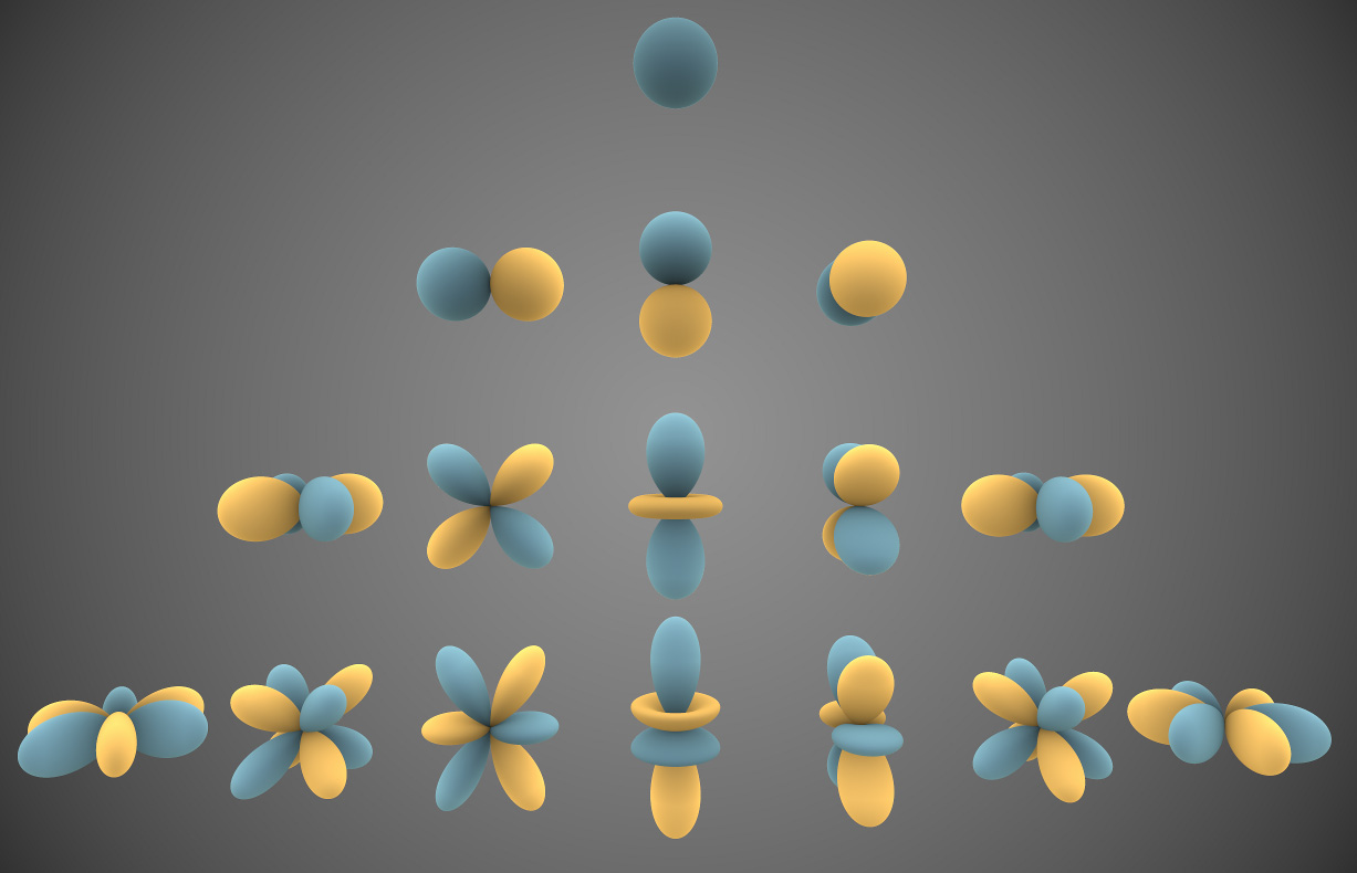
It is important to understand the general structure and symmetry of these functions, and in such matters, pictures are invaluable. Since the spherical harmonics with m 0 are complex, the most popular way of their graphical representation is to normalize their real and imaginary parts as
m
Im Y m
l
sin m , for m ,0
Y 2
(3.177)
lm
1 Re Y m
l
cos m , for m ,0
(for m = 0, Y
0
l 0 Yl ), and then plot the magnitude of these real functions72 in the spherical coordinates as the distance from the origin, while using two colors to show their sign – see Fig. 20.
Let us start from the simplest case l = 0. According to Eq. (162), for this lowest orbital quantum number, there may be only one magnetic quantum number: m = 0, and according to Eq. (174), the spherical harmonic corresponding to that state is just a constant. Thus the wavefunction of this so-called s state 73 is uniformly distributed over the sphere. Since this function has no gradient in any angular direction, it is only natural that the angular kinetic energy (163) of a particle in this state equals zero.
According to the same Eq. (162), for l = 1, there are 3 different p states, with m = –1, m = 0, and m = +1 – see Eq. (175). As the second row of Fig. 20 shows, these states are essentially identical in structure and are just differently oriented in space, thus readily explaining the 3-fold degeneracy of the kinetic energy (163).
72 Such real functions Ylm, which also form a full orthonormal set, and are frequently called the real (or “tesseral”) spherical harmonics, are more convenient than the complex harmonics Y m l for several applications, especially
when the variables of interest are real by definition.
73 The letter names for the states with various values of l stem from the history of optical spectroscopy – for example, the letter “s” (used for states with l = 0) originally denoted the “sharp” optical line series, etc. The sequence of the letters is as follows: s, p, d, f, g, and then continuing in alphabetical order.
Chapter 3
Page 40 of 64
Essential Graduate Physics
QM: Quantum Mechanics
Such a simple explanation, however, is not valid for the 5 different d states ( l = 2), shown in the third row of Fig. 20, as well as the states with higher l: despite their equal energies, they differ not only by their spatial orientation but their structure as well. All states with m = 0 have a nonzero gradient only in the direction. On the contrary, the states with the ultimate values of m ( l), change only monotonically (as sin l) in the polar direction, while oscillating in the azimuthal direction. The states with intermediate values of m provide a gradual transition between these two extremes, oscillating in both directions, stronger and stronger in the azimuthal direction as m is increased. Still, the magnetic quantum number, surprisingly, does not affect the angular energy for any l.
l = 0
( s state)
l = 1
( p states)
l = 2
( d states)
l = 3
( f
states)
m = –3
–2
–1
0
+1 +2
+3
Fig. 3.20. Plots of several lowest real spherical harmonics Ylm. (Adapted from https://en.wikipedia.org/wiki/Spherical_harmonics under the CC BY-SA 3.0 license.) Another counter-intuitive feature of the spherical harmonics follows from the comparison of Eq.
(163) with the second of Eqs. (152), which, in classical mechanics, is valid for the total angular momentum as well. They coincide only if we interpret
2
2
L l( l )
1 ,
(3.178)
as the value of the total L 2 L2 , including the and components of the vector L, in the state with eigenfunction Y m
l . On the other hand, the structure (159) of the azimuthal component F() of the wavefunction is exactly the same as in 2D axially symmetric problems, implying that Eq. (139) still gives correct values Lz = m for the z-component of the angular momentum. This fact invites a question: why for any state with l > 0, ( Lz)2 = m22 l 22 is always less than L 2 = l( l + 1)2? In other words, what prevents the angular momentum vector to be fully aligned with the z-axis?
Chapter 3
Page 41 of 64
QM: Quantum Mechanics
Besides the difficulty of answering this question using the above formulas, this analysis (though mathematically complete), is as intellectually unsatisfactory as the harmonic oscillator analysis in Sec.
2.9. In particular, it does not explain the meaning of the extremely simple relations for the eigenvalues of the energy and the angular momentum, coexisting with rather complicated eigenfunctions.
We will obtain natural answers to all these questions and concerns in Sec. 5.6 below, and now let us proceed to the extension of our wave-mechanical analysis to the 3D motion in an arbitrary spherically symmetric potential (155). In this case, we have to use the full form of the Laplace operator in spherical coordinates.74 The variable separation procedure is an evident generalization of what we have done above, with the particular solutions of the type
R ( r)Θ( ) F (),
(3.179)
whose substitution into the stationary Schrödinger equation yields
2
1 d 2 dR 1 1 d
d Θ
1
1 d 2 F
r
sin
U ( r) E .
(3.180)
2
2
2
2 r
m
R dr
dr Θ sin d
d
sin F d
It is evident that the angular part of the left-hand side (the two last terms in the square brackets) separates from the radial part, and that for the former part, we get Eq. (156) again, with the only change, R r. This change does not affect the fact that the eigenfunctions of that equation are still the spherical harmonics (171), which obey Eq. (164). As a result, Eq. (180) gives the following equation for the radial function R( r):
2
1 d 2 dR
r
l l( )
1 U ( r) E .
(3.181a)
2 r 2
m
R dr
dr
Note that no information about the magnetic quantum number m has crept into this radial equation (besides setting the limitation (162) for the possible values of l) so it includes only the orbital quantum number l. The equation may be also rewritten in a form similar to Eq. (148): 2
2
1 d
dR
l( l )
1
2
E E E , with E
r
U r
and
E
, (3.181b)
r
,
r
2
,
2
2 r
m
R dr
dr
2 r
m
expressing the same separability of the particle’s energy in the central field into the radial and angular components as in classical mechanics – cf. Eqs. (151)-(152), and also Eq. (163). In particular, since the expectation value of the latter component cannot be negative at l 0, this means that the ground state of any spherically symmetric system is an s-state, with l = 0 and hence m = 0.
Let us explore the radial equation for the simple case of a 3D particle free to move inside the sphere of radius R – say, confined there by the potential75
,
0
0
for
r R,
U
(3.182)
,
for
R r
.
In this case, Eq. (181a) is reduced to
74 Again, see MA Eq. (10.9).
75 This problem, besides giving a simple example of the quantization in spherically symmetric systems, is also an important precursor for the discussion of scattering by spherically symmetric potentials in Sec. 8.
Chapter 3
Page 42 of 64
QM: Quantum Mechanics
2
1 d dR
2
r
l( l )
1 E.
(3.183)
2
2
r
m
R dr
dr
Multiplying both parts of this equality by r 2 R, and introducing the dimensionless argument kr, where k 2 is defined by the usual relation 2 k 2/2m = E, we obtain the canonical form of this equation, 2
d
d
2
R
2
R
l l R
(3.184)
2
2 1
,
0
d
d
which is satisfied with the so-called spherical Bessel functions of the first and second kind, jl() and yl().76 These functions are directly related to the Bessel functions of semi-integer order,77
1/ 2
1/ 2
j ( )
J
( ),
y ( )
Y ( ),
(3.185)
l
2
1
l
l
2
1
l
2
2
but are actually much simpler than even the “usual” Bessel functions, such as Jn() and Yn() of an integer order n, because the former ones may be directly expressed via elementary functions: sin
sin
cos
3
1
3
j ( )
,
j ( )
,
j ( )
sin
cos ,...,
0
1
2
2
3
2
(3.186)
cos
cos
sin
3
1
3
y ( )
,
y ( )
,
y ( )
cos
sin ,...,
0
1
2
2
3
2
A few lowest-order spherical Bessel functions are plotted in Fig. 21.
1
0.5
l 0
l 0
1
2
3
0.5
0
1 2
j
3
y
l
l
0.5
0
0.5
1
0
5
10
15
0
5
10
15
Fig. 3.21. Several lowest-order spherical Bessel functions.
76 Alternatively, yl() are called “spherical Weber functions” or “spherical Neumann functions”.
77 Note that the Bessel functions J() and Y() of any order obey the universal recurrence relations and asymptotic formulas (discussed, e.g., in EM Sec. 2.7), so many properties of the functions jl() and yl() may be readily derived from these relations and Eqs. (185).
Chapter 3
Page 43 of 64
QM: Quantum Mechanics
As these formulas and plots show, the functions yl() are diverging at 0, and thus cannot be used in the solution of our current problem (182), so we have to take
R
const
.
(3.187)
l r
jl kr
Still, even for these functions, with the sole exception of the simplest function j 0(), the characteristic equation jl( kR) = 0, resulting from the boundary condition R( R)= 0, can be solved only numerically.
However, the roots l,n of the equation jl() = 0, where the integer n (= 1, 2, 3,…) is the root’s number, are tabulated in virtually any math handbook, and we may express the eigenvalues we are interested in, 2
2
2
2
k
l, n
l, n
l,
k
,
E
n
,