Information and Signal Theory by Anders Gjendemsjø, et al - HTML preview
Download the book in PDF, ePub for a complete version.
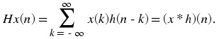
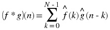
(2.1)
for all signals f, g defined on Z. It is important to note that the operation of convolution is
commutative, meaning that
(2.2)
f * g = g * f
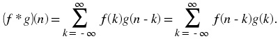
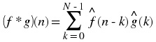
for all signals f, g defined on Z. Thus, the convolution operation could have been just as easily
stated using the equivalent definition
(2.3)
for all signals f, g defined on Z. Convolution has several other important properties not listed here but explained and derived in a later module.
Definition Motivation
The above operation definition has been chosen to be particularly useful in the study of linear time
invariant systems. In order to see this, consider a linear time invariant system H with unit impulse
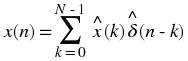
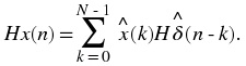
response h . Given a system input signal x we would like to compute the system output signal
H( x). First, we note that the input can be expressed as the convolution
(2.4)
by the sifting property of the unit impulse function. By linearity
(2.5)

Since H δ( n – k) is the shifted unit impulse response h( n – k), this gives the result (2.6)
Hence, convolution has been defined such that the output of a linear time invariant system is given
by the convolution of the system input with the system unit impulse response.
Graphical Intuition
It is often helpful to be able to visualize the computation of a convolution in terms of graphical
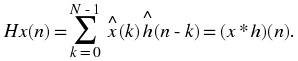
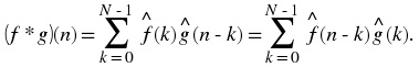
processes. Consider the convolution of two functions f, g given by
(2.7)
The first step in graphically understanding the operation of convolution is to plot each of the
functions. Next, one of the functions must be selected, and its plot reflected across the k = 0 axis.
For each real t , that same function must be shifted left by t . The product of the two resulting
plots is then constructed. Finally, the area under the resulting curve is computed.
Example 2.1.
Recall that the impulse response for a discrete time echoing feedback system with gain a is
(2.8)
h ( n ) = a n u ( n ) ,
and consider the response to an input signal that is another exponential
(2.9)
x ( n ) = b n u ( n ) .
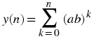
We know that the output for this input is given by the convolution of the impulse response
with the input signal
(2.10)
y ( n ) = x ( n ) * h ( n ) .
We would like to compute this operation by beginning in a way that minimizes the algebraic
complexity of the expression. However, in this case, each possible coice is equally simple.
Thus, we would like to compute
(2.11)
The step functions can be used to further simplify this sum. Therefore,
(2.12)
y ( n ) = 0
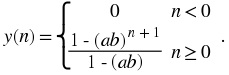


for n < 0 and
(2.13)
for n ≥ 0. Hence, provided a b ≠ 1, we have that
(2.14)
Circular Convolution
Discrete time circular convolution is an operation on two finite length or periodic discrete time
signals defined by the integral
(2.15)
for all signals f, g defined on Z[0, N – 1] where
are periodic extensions of f and g . It is
important to note that the operation of circular convolution is commutative, meaning that
(2.16)
f * g = g * f
for all signals f, g defined on Z[0, N – 1]. Thus, the circular convolution operation could have been just as easily stated using the equivalent definition
(2.17)
for all signals f, g defined on Z[0, N – 1] where
are periodic extensions of f and g . Circular
convolution has several other important properties not listed here but explained and derived in a
later module.
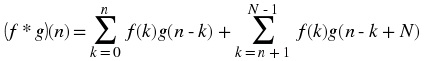
Alternatively, discrete time circular convolution can be expressed as the sum of two summations
given by
(2.18)
for all signals f, g defined on Z[0, N – 1].
Meaningful examples of computing discrete time circular convolutions in the time domain would
involve complicated algebraic manipulations dealing with the wrap around behavior, which would
ultimately be more confusing than helpful. Thus, none will be provided in this section. Of course,
example computations in the time domain are easy to program and demonstrate. However, disrete
time circular convolutions are more easily computed using frequency domain tools as will be
shown in the discrete time Fourier series section.
Definition Motivation
The above operation definition has been chosen to be particularly useful in the study of linear time
invariant systems. In order to see this, consider a linear time invariant system H with unit impulse
response h . Given a finite or periodic system input signal x we would like to compute the system
output signal H( x). First, we note that the input can be expressed as the circular convolution
(2.19)
by the sifting property of the unit impulse function. By linearity,
(2.20)
Since H δ( n – k) is the shifted unit impulse response h( n – k), this gives the result (2.21)
Hence, circular convolution has been defined such that the output of a linear time invariant system
is given by the convolution of the system input with the system unit impulse response.
Graphical Intuition
It is often helpful to be able to visualize the computation of a circular convolution in terms of
graphical processes. Consider the circular convolution of two finite length functions f, g given by (2.22)
The first step in graphically understanding the operation of convolution is to plot each of the
periodic extensions of the functions. Next, one of the functions must be selected, and its plot
reflected across the k = 0 axis. For each k ∈ Z[0, N – 1], that same function must be shifted left by k . The product of the two resulting plots is then constructed. Finally, the area under the resulting
curve on Z[0, N – 1] is computed.
Interactive Element
Figure 2.1.
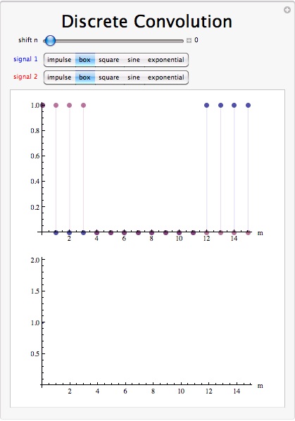
Interact (when online) with the Mathematica CDF demonstrating Discrete Linear Convolution. To download, right click and save file as .cdf
Convolution Summary
Convolution, one of the most important concepts in electrical engineering, can be used to
determine the output signal of a linear time invariant system for a given input signal with
knowledge of the system's unit impulse response. The operation of discrete time convolution is
defined such that it performs this function for infinite length discrete time signals and systems.
The operation of discrete time circular convolution is defined such that it performs this function
for finite length and periodic discrete time signals. In each case, the output of the system is the
convolution or circular convolution of the input signal with the unit impulse response.
2.3. Convolution - Analog*
In this module we examine convolution for continuous time signals. This will result in the
convolution integral and its properties. These concepts are very important in Electrical
Engineering and will make any engineer's life a lot easier if the time is spent now to truly
understand what is going on.
In order to fully understand convolution, you may find it useful to look at the discrete-time
convolution as well. Accompanied to this module there is a fully worked out example with
mathematics and figures. It will also be helpful to experiment with the Convolution - Continuous
time applet available from Johns Hopkins University. These resources offers different
approaches to this crucial concept.
Derivation of the convolution integral
The derivation used here closely follows the one discussed in the motivation section above. To
begin this, it is necessary to state the assumptions we will be making. In this instance, the only
constraints on our system are that it be linear and time-invariant.
Brief Overview of Derivation Steps:
1. An impulse input leads to an impulse response output.
2. A shifted impulse input leads to a shifted impulse response output. This is due to the time-
invariance of the system.
3. We now scale the impulse input to get a scaled impulse output. This is using the scalar
multiplication property of linearity.
4. We can now "sum up" an infinite number of these scaled impulses to get a sum of an infinite
number of scaled impulse responses. This is using the additivity attribute of linearity.
5. Now we recognize that this infinite sum is nothing more than an integral, so we convert both
sides into integrals.
6. Recognizing that the input is the function f( t) , we also recognize that the output is exactly the convolution integral.
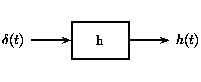
Figure 2.2.
We begin with a system defined by its impulse response, h( t) .
Figure 2.3.
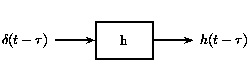

We then consider a shifted version of the input impulse. Due to the time invariance of the system, we obtain a shifted version of the output impulse response.
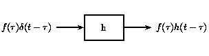
Figure 2.4.
Now we use the scaling part of linearity by scaling the system by a value, f( τ) , that is constant with respect to the system variable, t .
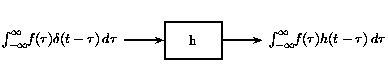
Figure 2.5.
We can now use the additivity aspect of linearity to add an infinite number of these, one for each possible τ . Since an infinite sum is exactly an integral, we end up with the integration known as the Convolution Integral. Using the sampling property, we recognize the left-hand side simply as the input f( t) .
Convolution Integral
As mentioned above, the convolution integral provides an easy mathematical way to express the
output of an LTI system based on an arbitrary signal, x( t) , and the system's impulse response,
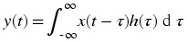
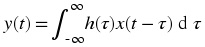
h( t) . The convolution integral is expressed as
Convolution is such an
important tool that it is represented by the symbol *, and can be written as y( t) = x( t) * h( t) By making a simple change of variables into the convolution integral, τ = t − τ , we can easily show that convolution is commutative: x( t) * h( t) = h( t) * x( t) which gives an equivivalent form of
For more information on the characteristics of the convolution
integral, read about the Properties of Convolution.
Implementation of Convolution
Taking a closer look at the convolution integral, we find that we are multiplying the input signal
by the time-reversed impulse response and integrating. This will give us the value of the output at

one given value of t . If we then shift the time-reversed impulse response by a small amount, we
get the output for another value of t . Repeating this for every possible value of t , yields the total output function. While we would never actually do this computation by hand in this fashion, it
does provide us with some insight into what is actually happening. We find that we are essentially
reversing the impulse response function and sliding it across the input function, integrating as we
go. This method, referred to as the graphical method, provides us with a much simpler way to
solve for the output for simple (contrived) signals, while improving our intuition for the more
complex cases where we rely on computers. In fact Texas Instruments develops Digital Signal
Processors which have special instruction sets for computations such as convolution.
Summary
Convolution is a truly important concept, which must be well understood.
Convoltion integral
Convoltion integral
Go to? Introduction; Convolution - Full example; Convolution - Discrete time; Properties of
2.4. Convolution - Complete example*
Basic Example
Let us look at a basic continuous-time convolution example to help express some of the important
ideas. We will convolve together two square pulses, x( t) and h( t), as shown in Figure 2.6
Figure 2.6.
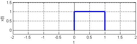
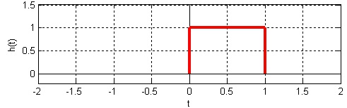
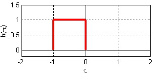
(a)
(b)
Two basic signals that we will convolve together.
Reflect and Shift
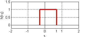
Now we will take one of the functions and reflect it around the y-axis. Then we must shift the
function, such that the origin, the point of the function that was originally on the origin, is labeled
as point t . This step is shown in Figure 2.7, h( t − τ) .
Figure 2.7.
(a) Reflected square pulse.
(b) Reflected and shifted square pulse.
h( – τ) and h( t − τ) .
Note that in Figure 2.7 τ is the 1st axis variable while t is a constant (in this figure). Since convolution is commutative it will never matter which function is reflected and shifted; however,
as the functions become more complicated reflecting and shifting the "right one" will often make
the problem much easier.
Regions of Integration
We start out with the convolution integral,
. The value of the function y at time
t is given by the amount of overlap(to be precise the integral of the overlapping region) between
h( t − τ) and x( τ) .
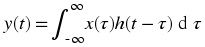
Next, we want to look at the functions and divide the span of the functions into different limits of
integration. These different regions can be understood by thinking about how we slide
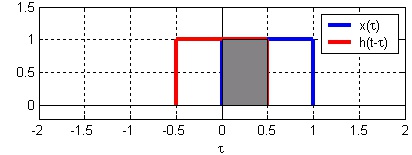
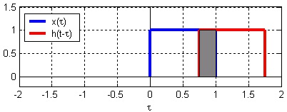
h( t − τ) over x( τ) , see Figure 2.8.
Figure 2.8.
(a) No overlap.
(b) h( t − τ) on its way "into" x( τ)
(c) h( t − τ) on its way "out of" x( τ)
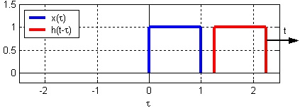
(d) No overlap.
Figures to help understand the regions of intergration
In this case we will have the following four regions. Compare these limits of integration to the
four illustrations of h( t − τ) and x( τ) in Figure 2.8.
Four Limits of Integration
1. t < 0
2. 0 ≤ t < 1
3. 1 ≤ t < 2
4. t ≥ 2
Using the Convolution Integral
Finally we are ready for a little math. Using the convolution integral, let us integrate the product
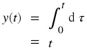
of x( τ) h( t − τ) . For our first and fourth region this will be trivial as it will always be 0. The second region, 0 ≤ t < 1 , will require the following math:
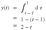
The third region, 1 ≤ t < 2 ,
is solved in much the same manner. Take note of the changes in our integration though. As we
move h( t − τ) across our other function, the left-hand edge of the function, t − 1 , becomes our lowlimit for the integral. This is shown through our convolution integral as
The
above formulas show the method for calculating convolution; however, do not let the simplicity of
this example confuse you when you work on other problems. The method will be the same, you
will just have to deal with more math in more complicated integrals.
Note that the value of y( t) at all time is given by the integral of the overlapping functions. In this example y for a given t equals the gray area in the plots in Figure 2.8.
Convolution Results

Thus, we have the following results for our four regions:
Now that we have found the
resulting function for each of the four regions, we can combine them together and graph the
convolution of x( t) * h( t) .
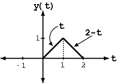
Figure 2.9.
Shows the system's output in response to the input, x( t) .
Common sense approach
By looking at Figure 2.8 we can obtain the system output, y( t), by "common" sense. For t < 0 there is no overlap, so y( t) is 0. As t goes from 0 to 1 the overlap will linearly increase with a maximum for t = 1, the maximum corresponds to the peak value in the triangular pulse. As t goes from 1 to 2
the overlap will linearly decrease. For t > 2 there will be no overlap and hence no output.
We see readily from the "common" sense approach that the output function y( t) is the same as obtained above with calculations. When convolving to square pulses the result will always be a
triangular pulse. Its origin, peak value and strech wi