Information and Signal Theory by Anders Gjendemsjø, et al - HTML preview
Download the book in PDF, ePub for a complete version.
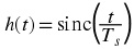
reconstruction formula, so that we can recover x( t) from x s ( n).
Proof part II - Signal reconstruction

Proof part II - Signal reconstruction
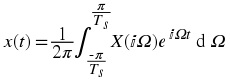
For a bandlimited signal the inverse fourier transform is
In the interval we
are integrating we have:
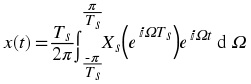
. Substituting this relation into Equation we get
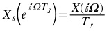
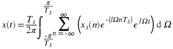
Using the DTFT relation for X s ( ⅇ ⅈ Ω T s ) we have Interchanging integration and summation (under the assumption of
convergence) leads to
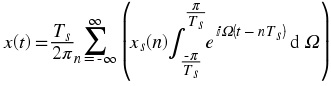
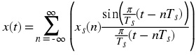
Finally we perform the integration and arrive
at the important reconstruction formula
(Thanks to R.Loos for pointing
out an error in the proof.)
Summary
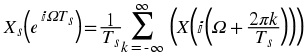
Spectrum sampled signal
Reconstruction formula
Go to Introduction; Illustrations; Matlab Example; Hold operation; Aliasing applet; System
4.3. Illustrations*
In this module we illustrate the processes involved in sampling and reconstruction. To see how all
these processes work together as a whole, take a look at the system view. In Sampling and
reconstruction with Matlab we provide a Matlab script for download. The matlab script shows the process of sampling and reconstruction live.
Basic examples
Example 4.1.
To sample an analog signal with 3000 Hz as the highest frequency component requires
sampling at 6000 Hz or above.
Example 4.2.
The sampling theorem can also be applied in two dimensions, i.e. for image analysis. A 2D
sampling theorem has a simple physical interpretation in image analysis: Choose the sampling
interval such that it is less than or equal to half of the smallest interesting detail in the image.
The process of sampling
We start off with an analog signal. This can for example be the sound coming from your stereo at
home or your friend talking.
The signal is then sampled uniformly. Uniform sampling implies that we sample every
T s seconds. In Figure 4.2 we see an analog signal. The analog signal has been sampled at times t = n T s .
Figure 4.2.
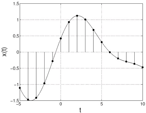


Analog signal, samples are marked with dots.
In signal processing it is often more convenient and easier to work in the frequency domain. So
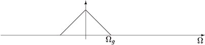
let's look at at the signal in frequency domain, Figure 4.3. For illustration purposes we take the frequency content of the signal as a triangle. (If you Fourier transform the signal in Figure 4.2 you will not get such a nice triangle.)
Figure 4.3.
The spectrum X( ⅈΩ) .
Notice that the signal in Figure 4.3 is bandlimited. We can see that the signal is bandlimited because X( ⅈΩ) is zero outside the interval [ – Ω g , Ω g ] . Equivalentely we can state that the signal has no angular frequencies above Ω g , corresponding to no frequencies above
.
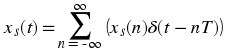
Now let's take a look at the sampled signal in the frequency domain. While proving the sampling theorem we found the the spectrum of the sampled signal consists of a sum of shifted versions of
the analog spectrum. Mathematically this is described by the following equation:


Sampling fast enough
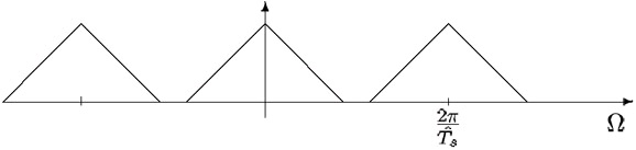
In Figure 4.4 we show the result of sampling x( t) according to the sampling theorem. This means that when sampling the signal in Figure 4.2/Figure 4.3 we use F s ≥ 2 F g . Observe in Figure 4.4
that we have the same spectrum as in Figure 4.3 for Ω ∈ [-Ω g , Ω g ] , except for the scaling factor
. This is a consequence of the sampling frequency. As mentioned in the proof the spectrum of the sampled signal is periodic with period
.
Figure 4.4.
The spectrum X s . Sampling frequency is OK.
So now we are, according to the sample theorem, able to reconstruct the original signal exactly.
How we can do this will be explored further down under reconstruction. But first we will take a look at what happens when we sample too slowly.
Sampling too slowly
If we sample x( t) too slowly, that is F s < 2 F g , we will get overlap between the repeated spectra, see Figure 4.5. According to Equation the resulting spectra is the sum of these. This overlap gives rise to the concept of aliasing.
Aliasing
If the sampling frequency is less than twice the highest frequency component, then
frequencies in the original signal that are above half the sampling rate will be
"aliased" and will appear in the resulting signal as lower frequencies.
The consequence of aliasing is that we cannot recover the original signal, so aliasing has to be
avoided. Sampling too slowly will produce a sequence x s ( n) that could have orginated from a number of signals. So there is no chance of recovering the original signal. To learn more about
aliasing, take a look at this module. (Includes an applet for demonstration!)
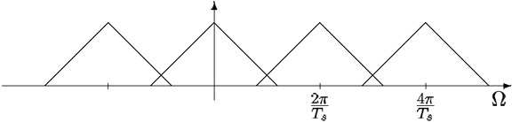
Figure 4.5.
The spectrum X s . Sampling frequency is too low.
To avoid aliasing we have to sample fast enough. But if we can't sample fast enough (possibly due
to costs) we can include an Anti-Aliasing filter. This will not able us to get an exact reconstruction
but can still be a good solution.
Anti-Aliasing filter
Typically a low-pass filter that is applied before sampling to ensure that no
components with frequencies greater than half the sample frequency remain.
Example 4.3.
The stagecoach effect
In older western movies you can observe aliasing on a stagecoach when it starts to roll. At
first the spokes appear to turn forward, but as the stagecoach increase its speed the spokes
appear to turn backward. This comes from the fact that the sampling rate, here the number of
frames per second, is too low. We can view each frame as a sample of an image that is
changing continuously in time. (Applet illustrating the stagecoach effect) Reconstruction
Given the signal in Figure 4.4 we want to recover the original signal, but the question is how?
When there is no overlapping in the spectrum, the spectral component given by k = 0 (see
Equation),is equal to the spectrum of the analog signal. This offers an oppurtunity to use a simple reconstruction process. Remember what you have learned about filtering. What we want is to
change signal in Figure 4.4 into that of Figure 4.3. To achieve this we have to remove all the extra components generated in the sampling process. To remove the extra components we apply an ideal
analog low-pass filter as shown in Figure 4.6 As we see the ideal filter is rectangular in the
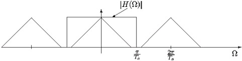
frequency domain. A rectangle in the frequency domain corresponds to a sinc function in time domain (and vice versa).
Figure 4.6.
H( ⅈΩ) The ideal reconstruction filter.
Then we have reconstructed the original spectrum, and as we know if two signals are identical in
the frequency domain, they are also identical in the time domain. End of reconstruction.
Conclusions
The Shannon sampling theorem requires that the input signal prior to sampling is band-limited to
at most half the sampling frequency. Under this condition the samples give an exact signal
representation. It is truly remarkable that such a broad and useful class signals can be represented
that easily!
We also looked into the problem of reconstructing the signals form its samples. Again the
simplicity of the principle is striking: linear filtering by an ideal low-pass filter will do the job.
However, the ideal filter is impossible to create, but that is another story...
Go to? Introduction; Proof; Illustrations; Matlab Example; Aliasing applet; Hold operation;
4.4. Sampling and reconstruction with Matlab*
Matlab files
Introduction; Proof; Illustrations; Aliasing applet; Hold operation; System view; Exercises
4.5. Aliasing Applet*

The applet is courtesy of the Digital Signal Processing tutorial at freeuk.com,
http://www.dsptutor.freeuk.com/. You can also have a look at the Light Wheel applet.
Introduction
In this module we shall look at sampling a sinusoidal signal. According to the sampling theorem, a sinusoidal signal can be exactly reconstructed from values sampled at discrete, uniform intervals
as long as the signal frequency is less than half the sampling frequency. Any component of a
sampled signal with a frequency above this limit, often referred to as the folding frequency, is
subject to aliasing.
The applet is based on a fixed sampling rate of F s = 8000 samples per second (one sample every
0.125 milliseconds, i.e
).
Instructions
Set the frequency of the sinusoidal signal, in Hz, in the "Input frequency" box, i.e choose an f in the following signal: sin(2 π f t) . When you click the "Plot" button, with "Input signal" checked, the input signal is plotted against time.
The "Grid" checkbox toggles on and off vertical gridlines indicating the instants at which the
signal is sampled. The "Sample points", representing the sampled values of the input signal, can
also be toggled.
Finally, the "Alias frequency" checkbox (visible only when aliasing occurs) controls the plotting of the "reconstructed" sinusoidal signal, with f = f alias .
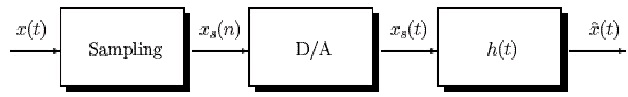
Overview of the process
When using the applet it is important to have an understanding of where the different signals
occur in a sampling system.
Figure 4.7.
Ideal sampling process

Relating the applet signals to the figure we get
Input signal = x( t) = sin(2 π f t) , where f is the input frequency chosen by the user.
The sampled signal =
.
The reconstructed signal = , is shown as the original signal if sampling is done fast enough, or
as the aliased signal if sampling is too slow.
( h( t) is an ideal reconstruction filter).
Aliasing demo applet
(This media type is not supported in this reader. Click to open media in browser.)
4.6. Hold operation*
Any practical reconstruction system must input finite length pulses into the reconstruction filter.
The reason is that we need nonzero energy in the nonzero pulses.
Introduction
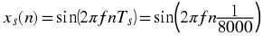
The operation performed to produce these pulses is called hold. Using the hold-operation we get
pulses with a predefined length and height proportional to the input to the digital-to-analog
converter. By means of the hold operation we get nonzero pulses with energy.
Figure 4.8.
Output signal from the hold device
As we have made changes relative to the ideal reconstruction, we need to look at the output signal the reconstruction filter will give us. Quite obviously the output will not be the original
signal. So, is it still useful?


Analysis
As before, and as will be the situation later, using the frequency domain simplifies the analysis.
To model the hold operation we use convolution with a delta function and a square pulse. The square pulse has unit height and duration τ . The duration τ is the holding time, i.e. how long we hold the incoming value. For the pulses not to overlap we must choose τ < T s . The convolution
can be seen as a filtering operation, using the square pulse as the impulse response. If we fourier
transform the square pulse we obtain the frequency response of the filter, which is a sinc
function.
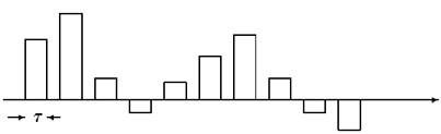
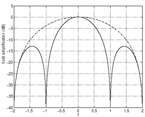
Figure 4.9 shows the frequency response of the analog square pulse filter. We have plotted the frequency response for τ = T s and
.
Figure 4.9.
Frequency response of the analog square filter as a function of digital frequency f.
From the figure we can make the following observations
The signal will be attenuated more and more towards the band edge, f = 0.5
For τ = T s the maximum attenuation is 3 dB at f = 0.5.
For
the maximum attenuation is 0.82 dB at f = 0.5.
The distortion is a result of linear operations and can thus be compensated for by using a filter
with opposite frequency response in the passband, f ∈ [ – 0.5, 0.5] . The compensation will not be
exact, but we can make the approximation as accurate as we wish. The compensation can be made
in the reconstruction filter or after the reconstruction by using a separate analog filter. One can
also predistort the signal in a digital filter before reconstruction. Where to put the compensator
and it's quality are cost considerations.


Go to? Introduction; Proof; Illustrations; Aliasing applet; System view; Exercises
4.7. Systems view of sampling and reconstruction*
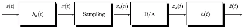
Ideal reconstruction system
Figure 4.10 shows the ideal reconstruction system based on the results of the Sampling theorem
Figure 4.10 consists of a sampling device which produces a time-discrete sequence x s ( n). The reconstruction filter, h( t), is an ideal analog sinc filter, with
. We can't apply the time-
discrete sequence x s ( n) directly to the analog filter h( t). To solve this problem we turn the sequence into an analog signal using delta functions. Thus we write
.
Figure 4.10.
Ideal reconstruction system
But when will the system produce an output
? According to the sampling theorem we
have
when the sampling frequency, F s , is at least twice the highest frequency component
of x( t).
Ideal system including anti-aliasing
To be sure that the reconstructed signal is free of aliasing it is customary to apply a lowpass filter,
an anti-aliasing filter, before sampling as shown in Figure 4.11.
Figure 4.11.
Ideal reconstruction system with anti-aliasing filter


Again we ask the question of when the system will produce an output
? If the signal is
entirely confined within the passband of the lowpass filter we will get perfect reconstruction if
F s is high enough.
But if the anti-aliasing filter removes the "higher" frequencies, (which in fact is the job of the
anti-aliasing filter), we will never be able to exactly reconstruct the original signal, s( t). If we sample fast enough we can reconstruct x( t), which in most cases is satisfying.
The reconstructed signal,
, will not have aliased frequencies. This is essential for further use
of the signal.
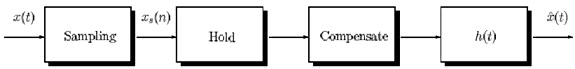
Reconstruction with hold operation
To make our reconstruction system realizable there are many things to look into. Among them are
the fact that any practical reconstruction system must input finite length pulses into the
reconstruction filter. This can be accomplished by the hold operation. To alleviate the distortion caused by the hold opeator we apply the output from the hold device to a compensator. The
compensation can be as accurate as we wish, this is cost and application consideration.
Figure 4.12.
More practical reconstruction system with a hold component
By the use of the hold component the reconstruction will not be exact, but as mentioned above we
can get as close as we want.
Introduction; Proof; Illustrations; Matlab example; Hold operation;