Information and Signal Theory by Anders Gjendemsjø, et al - HTML preview
Download the book in PDF, ePub for a complete version.
Information and Signal Theory
Collection edited by: Anders Gjendemsjø
Content authors: Anders Gjendemsjø, Melissa Selik, Richard Baraniuk, Ricardo Radaelli-
Sanchez, Stephen Kruzick, Catherine Elder, and Behnaam Aazhang
Online: < http://cnx.org/content/col10211/1.19>
This selection and arrangement of content as a collection is copyrighted by Anders Gjendemsjø.
It is licensed under the Creative Commons Attribution License: http://creativecommons.org/licenses/by/1.0
Collection structure revised: 2006/08/03
For copyright and attribution information for the modules contained in this collection, see the " Attributions" section at the end of the collection.
Information and Signal Theory
Table of Contents
1. Basic properties of signals
1. Basic properties of signals
2. Convolution
3. Analog Filtering
4. Sampling
5. Information theory
6. Decibel scale with signal processing applications
6. Decibel scale with signal processing applications
7. Filter types
8. Table of Formulas
9. Library
Cover Page
1. TTT4110: Information & Signal theory
Summary
Analysis and processing of signals that carry information. Representation of
signals in time and frequency domain.
Instructor: Bojana Gajic Scientific Assistants: Sebastien de la Ketthulle, Anders
Gjendemsjø Course Webpage: NTNU TTT4110
Welcome to TTT4110: Information & Signal Theory Connexions pages. At these pages we will present the following topics:
The material in these pages are partly based on the book Representing Information by
Signals,4th edition, by Tor Ramstad.
Chapter 1. Basic properties of signals
1.1. Introduction*
To describe signals and to understand that signals can carry information we need tools for
mathematical description and manipulation of signals.
In this chapter we introduce several important signals and show simple methods of describing
them. Depending on which type of signals we are looking at, it will be different methods
availiable for manipulating them. The elementary operations for manipulating signals and
sequences will be described.
Contents of this chapter
Introduction (current module)
Frequency definitions and periodicity
The simplest signals are one-dimensional and what follows is a classification of them.
Classification of signals
Analog signals
An analog signal is a continuous function of a continuous variable. Referring to Figure 1.1, this corresponds to that both the 1st AND the 2nd axis is continuous. The 1st axis will in general
correspond to the variable t , meaning time. In this context we define
signal range - the possible amplitude values the signal can take
signal axis - the time interval for which the signal exists
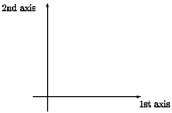
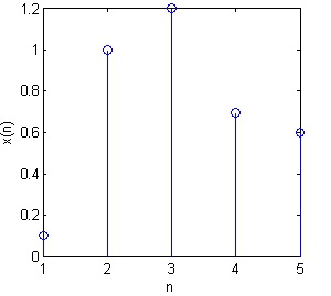
Figure 1.1.
Reference axes
Time discrete signals
A time discrete signal is a continuous signal of a discrete variable. Referring to Figure 1.1, we have the 1st axis discrete while the 2nd axis is continuous. Often we assign the values of the 1st
axis to a variable n . Time discrete signals often originate from analog signals being sampled.
More on that in the Sampling theorem chapter.
Figure 1.2.
Time discrete signal
Note that the signal is only defined for integer values along the 1st axis. We do not have any
information other than the values at index points.
Digital signals
Let the signal be a discrete function of a discrete variable, e.g. 1st and 2nd axis discrete, then the
signal will be digital. Examples of digital signals are a binary sequence. Digital signals often arise
from sampling analog signals and the samples being assigned to a discrete value.
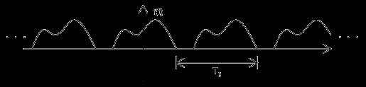
Periodic vs non periodic signals
All the signals mentioned above can be periodic. For time discrete and digital signals one has to
be extra cautious when "declaring" periodicity as we will see in Frequency definitions &
periodicity. Figure 1.3 shows a periodic signal with period T 0 and an aperiodic signal.
Figure 1.3.
(a) Periodic signal
(b) Aperiodic signal
(Figures by Melissa Selik)
Matlab file
Take a look at Discrete time signals; Analog signals; Discrete vs Analog signals; Frequency
definitions and periodicity; Energy & Power; Exercises ?
1.2. Discrete time signals*
The signals and relations presented in this module are quite similar to those in the Analog signals
module. So do compare and find similarities and differences!
Sequences
Generally a time discrete signal is a sequence of real or complex numbers. Each component in the
sequence is identified by an index: ...x(n-1),x(n), x(n+1),...
Example 1.1.
[x(n)] = [0.5 2.4 3.2 4.5] is a sequence. Using the index to identify a component we have
x(0) = 0.5 , x(1) = 2.4 and so on.
Manipulating sequences
Addition: Add individually each component with similar index
Multiplication by a constant: Multiply every component by the constant
Multiplication of sequences: Multiply each component individually
Delay: A delay by k implies that we shift the sequence by k. For this to make sense the sequence
has to be of infinite length.
Example 1.2.
Given the sequences [x(n)] = [0.5 2.4 3.2 4.5] and [y(n)] = [0.0 2.2 7.2 5.5].
a)Addition. [z(n)]=[x(n)]+[y(n)]=[0.5 4.6 10.4 10.0]
b)Multiplication by a constant c=2. [w(n)]= 2 *[x(n)] = [1.0 4.8 6.4 9.0]
Elementary signals & relations
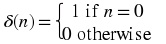
The unit sample
The unit sample is a signal which is zero everywhere except when its argument is zero, then it is
equal to 1. Mathematically
Unit sample
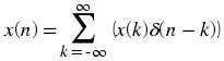
The unit sample function is very useful in that it can be seen as the elementary constituent in any
discrete signal. Let x( n) be a sequence. Then we can express x( n) as follows (using the unit sample definition and the delay operation)
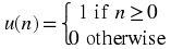
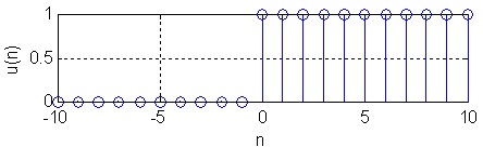
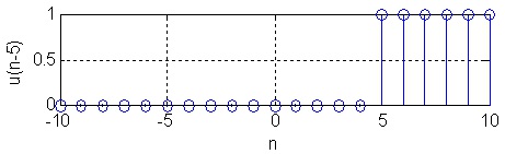
The unit step
The unit step function is equal to zero when its index is negative and equal to one for non-
negative indexes, see Figure 1.4 for plots.
Unit step
Figure 1.4.
(a) Unit step function, no delay.
(b) Unit step function, delayed by 5.
Two unit step functions.
Trigonometric functions
The discrete trigonometric functions are defined as follows. n is the sequence index and ω is the
angular frequency. ω = 2 π f , where f is the digital frequency.
Discrete sine
x( n) = sin( ωn)
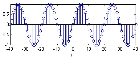

Discrete cosine
x( n) = cos( ωn)
Figure 1.5.
A discrete sine with digital frequency 1/20.
The complex exponential function
The complex exponential function is central to signal processing and some call it the most
important signal. Remember that it is a sequence and that
is the imaginary unit.
Complex exponential
x( n) = ⅇ ⅈωn
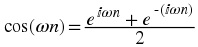
Euler's relations
The complex exponential function can be written as a sum of its real and imaginary part.
x( n) = ⅇ ⅈωn = cos( ωn) + ⅈ sin( ωn) By complex conjugating Equation and add / subtract the result with Equation we obtain Euler's relations.
Euler relation 1
Euler relation 2
The importance of Euler's relations can hardly be stressed enough.
Matlab files
Take a look at Introduction; Analog signals; Discrete vs Analog signals; Frequency definitions
and periodicity; Energy & Power; Exercises ?
1.3. Analog signals*
The signals signals and relations presented in this module are quite similar to those in the
Discrete time signals module. So do compare and find similarities and differences!
Manipulating signals
Mathematical operations on analog signals are unambiguous. We require that the signals are
defined over the same time interval when using operations such as addition, multiplication,
division and so on.
Elementary signals & relations
The (Dirac) delta function
The delta function is a peculiar function that has zero duration, infinite height, but still unit area!
Mathematically we have the following two properties
Delta function property I
δ( t) = 0 for t ≠ 0
Delta function property II
The delta function has a useful property, namely the sampling property.
At this
stage this may seem not particulary useful, so for now just convince yourself that the above
relation holds.
(We assume that x( t) is "well behaved" at t = τ , that is continuous and finite.) The unit step function
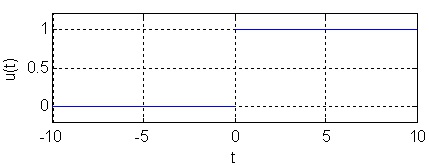
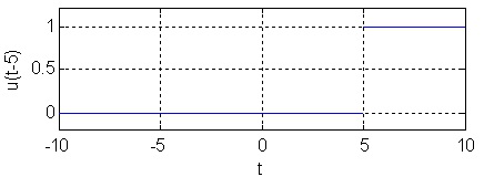
The unit step function is equal to zero when its argument is negative and equal to one for non-
negative arguments, see Figure 1.6 for plots.
Unit step
Figure 1.6.
(a) Unit step function, no delay.
(b) Unit step function, delayed by 5.
Two unit step functions.
Trigonometric functions
The trigonometric functions are central to signal processing and telecommunications. They are
defined as follows, where Ω is the angular frequency. Ω = 2 π F 0 , where F 0 is the frequency of the signal.
Sine
x( t) = sin( Ωt)

Cosine
x( t) = cos( Ωt)
See also Frequency definitions & periodicity.
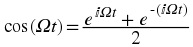
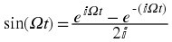
The complex exponential function
The complex exponential function is central to signal processing and some call it the most
important signal.
is the imaginary unit.
Complex exponential
x( t) = ⅇ ⅈΩt
Euler's relations
The complex exponential function can be written as a sum of its real and imaginary part.
x( t) = ⅇ ⅈΩt = cos( Ωt) + ⅈ sin( Ωt) By complex conjugating Equation and add / subtract the result with Equation we obtain Euler's relations.
Euler relation 1
Euler relation 2
The importance of Euler's relations can hardly be stressed enough.
Matlab file
Take a look at Introduction; Discrete time signals; Discrete vs Analog signals; Frequency
definitions and periodicity; Energy & Power; Exercises ?
1.4. Discrete vs Analog*
When comparing analog vs discrete time, we find that there are many similarities. Often we only
need to substitute the varible t with n and integration with summation. Still there are some
important differences that we need to know. As the complex exponential signal is truly central to
signal processing we will study that in more detail.
Analog
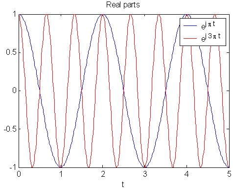
The complex exponential function is defined: x( t) = ⅇ ⅈΩt . If Ω(rad/second) is increased the rate of oscillation will increase continuously. The complex exponential function is also periodic for
any value of Ω. In figure Figure 1.7 we have plotted ⅇ ⅈπt and ⅇ ⅈ 3 π t (the real parts only). In
Figure 1.7 we see that the red plot, corresponding to a higher value of Ω, has a higher rate of oscillation.
Figure 1.7.
Real parts of complex exponentials.
Discrete time
The discrete time complex exponential function is defined: x( n) = ⅇ ⅈωn .
If we increase ω (rad/sample) the rate of oscillation will increase and decrease periodically. The
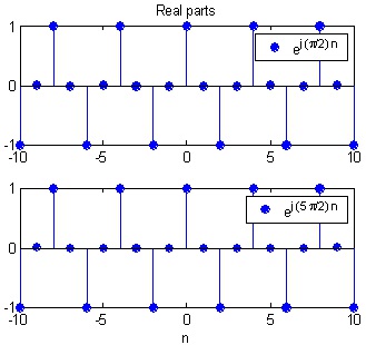
reason is: ⅇ ⅈ( ω + 2 π k) n = ⅇ ⅈωn ⅇ ⅈ 2 π k n = ⅇ ⅈωn , where n,k ∈ ℤ .
This implies that the complex exponential with digital angular frequency ω is identical to a
complex exponential with ω 1 = ω + 2 π , see Figure 1.8
Figure 1.8.
Two discrete exponentials that are identical
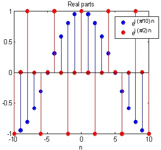
The rate of oscillation will increase until ω = π , then it decreases and repeats after 2π. In
Figure 1.9 we see that as we increase the angular frequency towards π the rate of oscillation increases. If you download the Matlab files included at the end of this module you can adjust the
parameters and see that the rate of oscillation will decrease when exceeding π (but less than 2π).
Figure 1.9.

Two discrete exponentials with different frequency.
Consequence
We need to consider discrete time exponentials at an (digital angular) frequency
interval of 2π only.
Low (digital angular) frequencies will correspond to ω near even multiplies of π. High (digital
angular) frequencies will correspond to ω near odd multiplies of π.
Matlab files
Take a look at Introduction; Discrete time signals; Analog signals; Frequency definitions and
periodicity; Energy & Power; Exercises ?
1.5. Frequency definitions and periodicity*
Frequency definitions
In signal processing we use several types of frequencies. This may seem confusing at first, but it
is really not that difficult.
Analog frequency
The frequency of an analog signal is the easiest to understand. A trigonometric function with
argument Ωt = 2 π F t generates a periodic function with
a single frequency F.
period T
the relation
Frequency is then interpreted as how many periods there are per time unit. If we choose seconds
as our time unit, frequency will be measured in Hertz, which is most common.

