bands.
• List and explain the different methods by which electromagnetic waves are produced across the spectrum.
24.4. Energy in Electromagnetic Waves
• Explain how the energy and amplitude of an electromagnetic wave are related.
• Given its power output and the heating area, calculate the intensity of a microwave oven’s electromagnetic field, as well as its peak
electric and magnetic field strengths
Introduction to Electromagnetic Waves
The beauty of a coral reef, the warm radiance of sunshine, the sting of sunburn, the X-ray revealing a broken bone, even microwave popcorn—all are
brought to us by electromagnetic waves. The list of the various types of electromagnetic waves, ranging from radio transmission waves to nuclear
gamma-ray ( γ -ray) emissions, is interesting in itself.
Even more intriguing is that all of these widely varied phenomena are different manifestations of the same thing—electromagnetic waves. (See
Figure 24.2.) What are electromagnetic waves? How are they created, and how do they travel? How can we understand and organize their widely
varying properties? What is their relationship to electric and magnetic effects? These and other questions will be explored.
862 CHAPTER 24 | ELECTROMAGNETIC WAVES
Misconception Alert: Sound Waves vs. Radio Waves
Many people confuse sound waves with radio waves, one type of electromagnetic (EM) wave. However, sound and radio waves are completely
different phenomena. Sound creates pressure variations (waves) in matter, such as air or water, or your eardrum. Conversely, radio waves are
electromagnetic waves, like visible light, infrared, ultraviolet, X-rays, and gamma rays. EM waves don’t need a medium in which to propagate;
they can travel through a vacuum, such as outer space.
A radio works because sound waves played by the D.J. at the radio station are converted into electromagnetic waves, then encoded and
transmitted in the radio-frequency range. The radio in your car receives the radio waves, decodes the information, and uses a speaker to change
it back into a sound wave, bringing sweet music to your ears.
Discovering a New Phenomenon
It is worth noting at the outset that the general phenomenon of electromagnetic waves was predicted by theory before it was realized that light is a
form of electromagnetic wave. The prediction was made by James Clerk Maxwell in the mid-19th century when he formulated a single theory
combining all the electric and magnetic effects known by scientists at that time. “Electromagnetic waves” was the name he gave to the phenomena
his theory predicted.
Such a theoretical prediction followed by experimental verification is an indication of the power of science in general, and physics in particular. The
underlying connections and unity of physics allow certain great minds to solve puzzles without having all the pieces. The prediction of
electromagnetic waves is one of the most spectacular examples of this power. Certain others, such as the prediction of antimatter, will be discussed
in later modules.
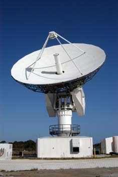
Figure 24.2 The electromagnetic waves sent and received by this 50-foot radar dish antenna at Kennedy Space Center in Florida are not visible, but help track expendable
launch vehicles with high-definition imagery. The first use of this C-band radar dish was for the launch of the Atlas V rocket sending the New Horizons probe toward Pluto.
(credit: NASA)
24.1 Maxwell’s Equations: Electromagnetic Waves Predicted and Observed
The Scotsman James Clerk Maxwell (1831–1879) is regarded as the greatest theoretical physicist of the 19th century. (See Figure 24.3.) Although
he died young, Maxwell not only formulated a complete electromagnetic theory, represented by Maxwell’s equations, he also developed the kinetic
theory of gases and made significant contributions to the understanding of color vision and the nature of Saturn’s rings.
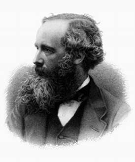
Figure 24.3 James Clerk Maxwell, a 19th-century physicist, developed a theory that explained the relationship between electricity and magnetism and correctly predicted that
visible light is caused by electromagnetic waves. (credit: G. J. Stodart)
Maxwell brought together all the work that had been done by brilliant physicists such as Oersted, Coulomb, Gauss, and Faraday, and added his own
insights to develop the overarching theory of electromagnetism. Maxwell’s equations are paraphrased here in words because their mathematical
statement is beyond the level of this text. However, the equations illustrate how apparently simple mathematical statements can elegantly unite and
express a multitude of concepts—why mathematics is the language of science.
CHAPTER 24 | ELECTROMAGNETIC WAVES 863
Maxwell’s Equations
1. Electric field lines originate on positive charges and terminate on negative charges. The electric field is defined as the force per unit
charge on a test charge, and the strength of the force is related to the electric constant ε 0 , also known as the permittivity of free space.
From Maxwell’s first equation we obtain a special form of Coulomb’s law known as Gauss’s law for electricity.
2. Magnetic field lines are continuous, having no beginning or end. No magnetic monopoles are known to exist. The strength of the magnetic
force is related to the magnetic constant µ 0 , also known as the permeability of free space. This second of Maxwell’s equations is known
as Gauss’s law for magnetism.
3. A changing magnetic field induces an electromotive force (emf) and, hence, an electric field. The direction of the emf opposes the change.
This third of Maxwell’s equations is Faraday’s law of induction, and includes Lenz’s law.
4. Magnetic fields are generated by moving charges or by changing electric fields. This fourth of Maxwell’s equations encompasses Ampere’s
law and adds another source of magnetism—changing electric fields.
Maxwell’s equations encompass the major laws of electricity and magnetism. What is not so apparent is the symmetry that Maxwell introduced in his
mathematical framework. Especially important is his addition of the hypothesis that changing electric fields create magnetic fields. This is exactly
analogous (and symmetric) to Faraday’s law of induction and had been suspected for some time, but fits beautifully into Maxwell’s equations.
Symmetry is apparent in nature in a wide range of situations. In contemporary research, symmetry plays a major part in the search for sub-atomic
particles using massive multinational particle accelerators such as the new Large Hadron Collider at CERN.
Making Connections: Unification of Forces
Maxwell’s complete and symmetric theory showed that electric and magnetic forces are not separate, but different manifestations of the same
thing—the electromagnetic force. This classical unification of forces is one motivation for current attempts to unify the four basic forces in
nature—the gravitational, electrical, strong, and weak nuclear forces.
Since changing electric fields create relatively weak magnetic fields, they could not be easily detected at the time of Maxwell’s hypothesis. Maxwell
realized, however, that oscillating charges, like those in AC circuits, produce changing electric fields. He predicted that these changing fields would
propagate from the source like waves generated on a lake by a jumping fish.
The waves predicted by Maxwell would consist of oscillating electric and magnetic fields—defined to be an electromagnetic wave (EM wave).
Electromagnetic waves would be capable of exerting forces on charges great distances from their source, and they might thus be detectable. Maxwell
calculated that electromagnetic waves would propagate at a speed given by the equation
(24.1)
c = 1
µ
.
0 ε 0
When the values for µ 0 and ε 0 are entered into the equation for c , we find that
(24.2)
c =
1
= 3.00×10⁸ m/s,
(8.85×10⁻¹² C2
N ⋅ m2)(4π × 10−7 T ⋅ m
A )
which is the speed of light. In fact, Maxwell concluded that light is an electromagnetic wave having such wavelengths that it can be detected by the
eye.
Other wavelengths should exist—it remained to be seen if they did. If so, Maxwell’s theory and remarkable predictions would be verified, the greatest
triumph of physics since Newton. Experimental verification came within a few years, but not before Maxwell’s death.
Hertz’s Observations
The German physicist Heinrich Hertz (1857–1894) was the first to generate and detect certain types of electromagnetic waves in the laboratory.
Starting in 1887, he performed a series of experiments that not only confirmed the existence of electromagnetic waves, but also verified that they
travel at the speed of light.
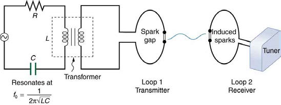
Hertz used an AC RLC (resistor-inductor-capacitor) circuit that resonates at a known frequency f 0 =
1
2π
and connected it to a loop of wire as
LC
shown in Figure 24.4. High voltages induced across the gap in the loop produced sparks that were visible evidence of the current in the circuit and that helped generate electromagnetic waves.
Across the laboratory, Hertz had another loop attached to another RLC circuit, which could be tuned (as the dial on a radio) to the same resonant
frequency as the first and could, thus, be made to receive electromagnetic waves. This loop also had a gap across which sparks were generated,
giving solid evidence that electromagnetic waves had been received.
864 CHAPTER 24 | ELECTROMAGNETIC WAVES
Figure 24.4 The apparatus used by Hertz in 1887 to generate and detect electromagnetic waves. An RLC circuit connected to the first loop caused sparks across a gap in
the wire loop and generated electromagnetic waves. Sparks across a gap in the second loop located across the laboratory gave evidence that the waves had been received.
Hertz also studied the reflection, refraction, and interference patterns of the electromagnetic waves he generated, verifying their wave character. He
was able to determine wavelength from the interference patterns, and knowing their frequency, he could calculate the propagation speed using the
equation υ = fλ (velocity—or speed—equals frequency times wavelength). Hertz was thus able to prove that electromagnetic waves travel at the
speed of light. The SI unit for frequency, the hertz ( 1 Hz = 1 cycle/sec ), is named in his honor.
24.2 Production of Electromagnetic Waves
We can get a good understanding of electromagnetic waves (EM) by considering how they are produced. Whenever a current varies, associated
electric and magnetic fields vary, moving out from the source like waves. Perhaps the easiest situation to visualize is a varying current in a long
straight wire, produced by an AC generator at its center, as illustrated in Figure 24.5.
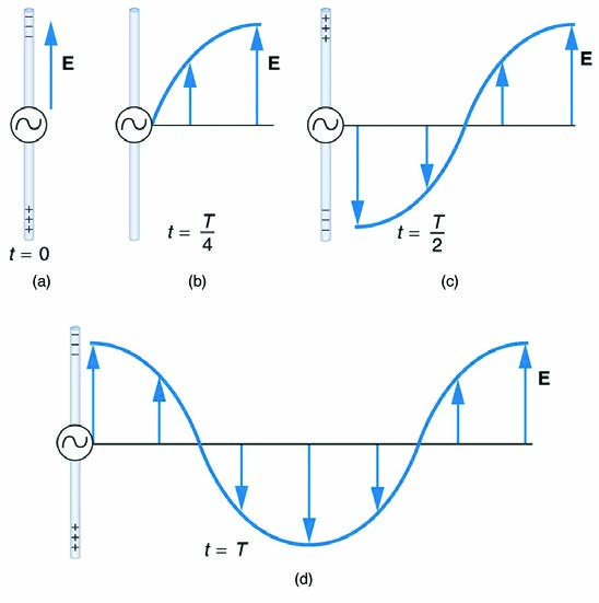
Figure 24.5 This long straight gray wire with an AC generator at its center becomes a broadcast antenna for electromagnetic waves. Shown here are the charge distributions
at four different times. The electric field ( E ) propagates away from the antenna at the speed of light, forming part of an electromagnetic wave.
The electric field ( E ) shown surrounding the wire is produced by the charge distribution on the wire. Both the E and the charge distribution vary as
the current changes. The changing field propagates outward at the speed of light.
There is an associated magnetic field ( B ) which propagates outward as well (see Figure 24.6). The electric and magnetic fields are closely related
and propagate as an electromagnetic wave. This is what happens in broadcast antennae such as those in radio and TV stations.
Closer examination of the one complete cycle shown in Figure 24.5 reveals the periodic nature of the generator-driven charges oscillating up and
down in the antenna and the electric field produced. At time t = 0 , there is the maximum separation of charge, with negative charges at the top and
positive charges at the bottom, producing the maximum magnitude of the electric field (or E -field) in the upward direction. One-fourth of a cycle later,
there is no charge separation and the field next to the antenna is zero, while the maximum E -field has moved away at speed c .
As the process continues, the charge separation reverses and the field reaches its maximum downward value, returns to zero, and rises to its
maximum upward value at the end of one complete cycle. The outgoing wave has an amplitude proportional to the maximum separation of charge.
Its wavelength ( λ) is proportional to the period of the oscillation and, hence, is smaller for short periods or high frequencies. (As usual, wavelength
and frequency ⎛⎝ f ⎞⎠ are inversely proportional.)

CHAPTER 24 | ELECTROMAGNETIC WAVES 865
Electric and Magnetic Waves: Moving Together
Following Ampere’s law, current in the antenna produces a magnetic field, as shown in Figure 24.6. The relationship between E and B is shown at one instant in Figure 24.6 (a). As the current varies, the magnetic field varies in magnitude and direction.
Figure 24.6 (a) The current in the antenna produces the circular magnetic field lines. The current ( I ) produces the separation of charge along the wire, which in turn creates the electric field as shown. (b) The electric and magnetic fields ( E and B ) near the wire are perpendicular; they are shown here for one point in space. (c) The magnetic field varies with current and propagates away from the antenna at the speed of light.
The magnetic field lines also propagate away from the antenna at the speed of light, forming the other part of the electromagnetic wave, as seen in
Figure 24.6 (b). The magnetic part of the wave has the same period and wavelength as the electric part, since they are both produced by the same
movement and separation of charges in the antenna.
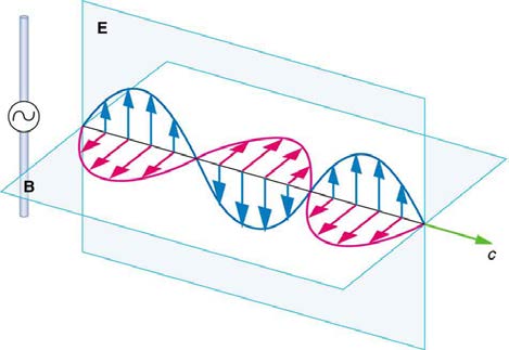
The electric and magnetic waves are shown together at one instant in time in Figure 24.7. The electric and magnetic fields produced by a long
straight wire antenna are exactly in phase. Note that they are perpendicular to one another and to the direction of propagation, making this a
transverse wave.
Figure 24.7 A part of the electromagnetic wave sent out from the antenna at one instant in time. The electric and magnetic fields ( E and B ) are in phase, and they are perpendicular to one another and the direction of propagation. For clarity, the waves are shown only along one direction, but they propagate out in other directions too.
Electromagnetic waves generally propagate out from a source in all directions, sometimes forming a complex radiation pattern. A linear antenna like
this one will not radiate parallel to its length, for example. The wave is shown in one direction from the antenna in Figure 24.7 to illustrate its basic characteristics.
Instead of the AC generator, the antenna can also be driven by an AC circuit. In fact, charges radiate whenever they are accelerated. But while a
current in a circuit needs a complete path, an antenna has a varying charge distribution forming a standing wave, driven by the AC. The dimensions
of the antenna are critical for determining the frequency of the radiated electromagnetic waves. This is a resonant phenomenon and when we tune
radios or TV, we vary electrical properties to achieve appropriate resonant conditions in the antenna.
Receiving Electromagnetic Waves
Electromagnetic waves carry energy away from their source, similar to a sound wave carrying energy away from a standing wave on a guitar string.
An antenna for receiving EM signals works in reverse. And like antennas that produce EM waves, receiver antennas are specially designed to
resonate at particular frequencies.
An incoming electromagnetic wave accelerates electrons in the antenna, setting up a standing wave. If the radio or TV is switched on, electrical
components pick up and amplify the signal formed by the accelerating electrons. The signal is then converted to audio and/or video format.
Sometimes big receiver dishes are used to focus the signal onto an antenna.
In fact, charges radiate whenever they are accelerated. When designing circuits, we often assume that energy does not quickly escape AC circuits,
and mostly this is true. A broadcast antenna is specially designed to enhance the rate of electromagnetic radiation, and shielding is necessary to
keep the radiation close to zero. Some familiar phenomena are based on the production of electromagnetic waves by varying currents. Your
microwave oven, for example, sends electromagnetic waves, called microwaves, from a concealed antenna that has an oscillating current imposed
on it.
Relating E -Field and B -Field Strengths
There is a relationship between the E - and B -field strengths in an electromagnetic wave. This can be understood by again considering the antenna
just described. The stronger the E -field created by a separation of charge, the greater the current and, hence, the greater the B -field created.
Since current is directly proportional to voltage (Ohm’s law) and voltage is directly proportional to E -field strength, the two should be directly
proportional. It can be shown that the magnitudes of the fields do have a constant ratio, equal to the speed of light. That is,

866 CHAPTER 24 | ELECTROMAGNETIC WAVES
E
(24.3)
B = c
is the ratio of E -field strength to B -field strength in any electromagnetic wave. This is true at all times and at all locations in space. A simple and
elegant result.
Example 24.1 Calculating B -Field Strength in an Electromagnetic Wave
What is the maximum strength of the B -field in an electromagnetic wave that has a maximum E -field strength of 1000 V/m ?
Strategy
To find the B -field strength, we rearrange the above equation to solve for B , yielding
(24.4)
B = Ec.
Solution
We are given E , and c is the speed of light. Entering these into the expression for B yields
(24.5)
B = 1000 V/m = 3.33×10⁻⁶ T,
3.00×10⁸ m/s
Where T stands for Tesla, a measure of magnetic field strength.
Discussion
The B -field strength is less than a tenth of the Earth’s admittedly weak magnetic field. This means that a relatively strong electric field of 1000
V/m is accompanied by a relatively weak magnetic field. Note that as this wave spreads out, say with distance from an antenna, its field
strengths become progressively weaker.
The result of this example is consistent with the statement made in the module Maxwell’s Equations: Electromagnetic Waves Predicted and
Observed that changing electric fields create relatively weak magnetic fields. They can be detected in electromagnetic waves, however, by taking
advantage of the phenomenon of resonance, as Hertz did. A system with the same natural frequency as the electromagnetic wave can be made to
oscillate. All radio and TV receivers use this principle to pick up and then amplify weak electromagnetic waves, while rejecting all others not at their
resonant frequency.
Take-Home Experiment: Antennas
For your TV or radio at home, identify the antenna, and sketch its shape. If you don’t have cable, you might have an outdoor or indoor TV
antenna. Estimate its size. If the TV signal is between 60 and 216 MHz for basic channels, then what is the wavelength of those EM waves?
Try tuning the radio and note the small range of frequencies at which a reasonable signal for that station is received. (This is easier with digital
readout.) If you have a car with a radio and extendable antenna, note the quality of reception as the length of the antenna is changed.
PhET Explorations: Radio Waves and Electromagnetic Fields
Broadcast radio waves from KPhET. Wiggle the transmitter electron manually or have it oscillate automatically. Display the field as a curve or
vectors. The strip chart shows the electron positions at the transmitter and at the receiver.
Figure 24.8 Radio Waves and Electromagnetic Fields (http://cnx.org/content/m42440/1.4/radio-waves_en.jar)
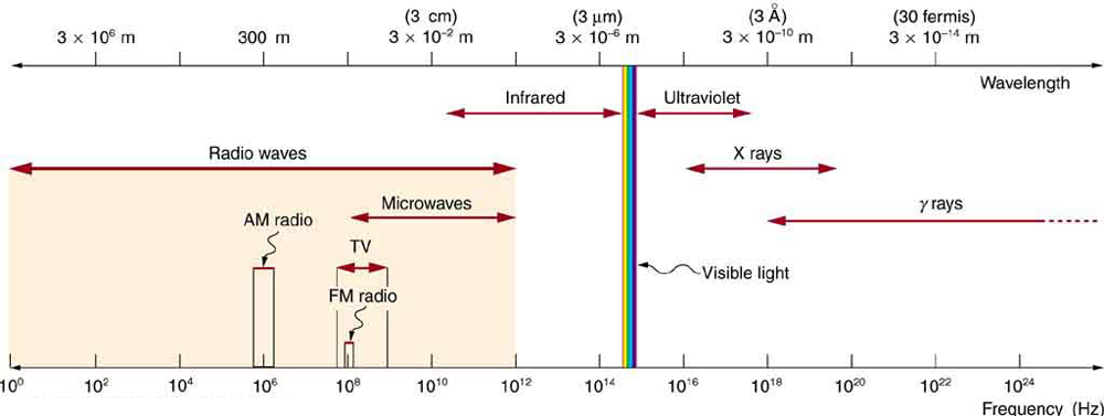
24.3 The Electromagnetic Spectrum
In this module we examine how electromagnetic waves are classified into categories such as radio, infrared, ultraviolet, and so on, so that we can
understand some of their similarities as well as some of their differences. We will also find that there are many connections with previously discussed
topics, such as wavelength and resonance. A brief overview of the production and utilization of electromagnetic waves is found in Table 24.1.
CHAPTER 24 | ELECTROMAGNETIC WAVES 867
Table 24.1 Electromagnetic Waves
Type of EM
Production
Applications
Life sciences aspect
Issues
wave
Communications Remote
Requires controls for band
Radio & TV
Accelerating charges
MRI
controls
use
Accelerating charges & thermal
Communications Ovens
Microwaves
Deep heating
Cell phone use
agitation
Radar
Thermal agitations & electronic
Infrared
Thermal imaging Heating
Absorbed by atmosphere
Greenhouse effect
transitions
Thermal agitations & electronic
Photosynthesis Human
Visible light
All pervasive
transitions
vision
Thermal agitations & electronic
Ozone depletion Cancer
Ultraviolet
Sterilization Cancer control
Vitamin D production
transitions
causing
Inner electronic transitions and fast
Medical diagnosis Cancer
X-rays
Medical Security
Cancer causing
collisions
therapy
Medical diagnosis Cancer
Cancer causing Radiation
Gamma rays
Nuclear decay
Nuclear medicineSecurity
therapy
damage
Connections: Waves
There are many types of waves, such as water waves and even earthquakes. Among the many shared attributes of waves are propagation
speed, frequency, and wavelength. These are always related by the expression v W = fλ . This module concentrates on EM waves, but other
modules contain examples of all of these characteristics for sound waves and submicroscopic particles.
As noted before, an electromagnetic wave has a frequency and a wavelength associated with it and travels at the speed of light, or c . The
relationship among these wave characteristics can be described by v W = fλ , where v W is the propagation speed of the wave, f is the frequency,
and
Describe what you're looking for in as much detail as you'd like.
Our AI reads your request and finds the best matching books for you.
Popular searches:
Join 2.9 million readers and get unlimited free ebooks