emf = BΔ A
Δ t = BℓΔ x
Δ t .
Finally, note that Δ x / Δ t = v , the velocity of the rod. Entering this into the last expression shows that
(23.9)
emf = Bℓv
( B, ℓ, and v perpendicular)
is the motional emf. This is the same expression given for the Hall effect previously.
Making Connections: Unification of Forces
There are many connections between the electric force and the magnetic force. The fact that a moving electric field produces a magnetic field
and, conversely, a moving magnetic field produces an electric field is part of why electric and magnetic forces are now considered to be different
manifestations of the same force. This classic unification of electric and magnetic forces into what is called the electromagnetic force is the
inspiration for contemporary efforts to unify other basic forces.
CHAPTER 23 | ELECTROMAGNETIC INDUCTION, AC CIRCUITS, AND ELECTRICAL TECHNOLOGIES 821
To find the direction of the induced field, the direction of the current, and the polarity of the induced emf, we apply Lenz’s law as explained in
Faraday's Law of Induction: Lenz's Law. (See Figure 23.11(b).) Flux is increasing, since the area enclosed is increasing. Thus the induced field
must oppose the existing one and be out of the page. And so the RHR-2 requires that I be counterclockwise, which in turn means the top of the rod is
positive as shown.
Motional emf also occurs if the magnetic field moves and the rod (or other object) is stationary relative to the Earth (or some observer). We have seen
an example of this in the situation where a moving magnet induces an emf in a stationary coil. It is the relative motion that is important. What is
emerging in these observations is a connection between magnetic and electric fields. A moving magnetic field produces an electric field through its
induced emf. We already have seen that a moving electric field produces a magnetic field—moving charge implies moving electric field and moving
charge produces a magnetic field.
Motional emfs in the Earth’s weak magnetic field are not ordinarily very large, or we would notice voltage along metal rods, such as a screwdriver,
during ordinary motions. For example, a simple calculation of the motional emf of a 1 m rod moving at 3.0 m/s perpendicular to the Earth’s field gives
emf = Bℓv = (5.0×10⁻⁵ T)(1.0 m)(3.0 m/s) = 150 μV . This small value is consistent with experience. There is a spectacular exception,
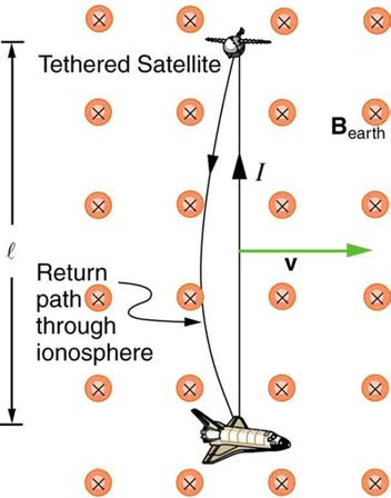
however. In 1992 and 1996, attempts were made with the space shuttle to create large motional emfs. The Tethered Satellite was to be let out on a
20 km length of wire as shown in Figure 23.12, to create a 5 kV emf by moving at orbital speed through the Earth’s field. This emf could be used to convert some of the shuttle’s kinetic and potential energy into electrical energy if a complete circuit could be made. To complete the circuit, the
stationary ionosphere was to supply a return path for the current to flow. (The ionosphere is the rarefied and partially ionized atmosphere at orbital
altitudes. It conducts because of the ionization. The ionosphere serves the same function as the stationary rails and connecting resistor in Figure
23.11, without which there would not be a complete circuit.) Drag on the current in the cable due to the magnetic force F = IℓB sin θ does the work that reduces the shuttle’s kinetic and potential energy and allows it to be converted to electrical energy. The tests were both unsuccessful. In the first,
the cable hung up and could only be extended a couple of hundred meters; in the second, the cable broke when almost fully extended. Example 23.2
indicates feasibility in principle.
Example 23.2 Calculating the Large Motional Emf of an Object in Orbit
Figure 23.12 Motional emf as electrical power conversion for the space shuttle is the motivation for the Tethered Satellite experiment. A 5 kV emf was predicted to be
induced in the 20 km long tether while moving at orbital speed in the Earth’s magnetic field. The circuit is completed by a return path through the stationary ionosphere.
Calculate the motional emf induced along a 20.0 km long conductor moving at an orbital speed of 7.80 km/s perpendicular to the Earth’s
5.00×10⁻⁵ T magnetic field.
Strategy
This is a straightforward application of the expression for motional emf— emf = Bℓv .
Solution
Entering the given values into emf = Bℓv gives
(23.10)
emf = Bℓv
= (5.00×10⁻⁵ T)(2.0×10⁴ m)(7.80×10³ m/s)
= 7.80×10³ V.
Discussion
The value obtained is greater than the 5 kV measured voltage for the shuttle experiment, since the actual orbital motion of the tether is not
perpendicular to the Earth’s field. The 7.80 kV value is the maximum emf obtained when θ = 90º and sin θ = 1 .
822 CHAPTER 23 | ELECTROMAGNETIC INDUCTION, AC CIRCUITS, AND ELECTRICAL TECHNOLOGIES
23.4 Eddy Currents and Magnetic Damping
Eddy Currents and Magnetic Damping
As discussed in Motional Emf, motional emf is induced when a conductor moves in a magnetic field or when a magnetic field moves relative to a
conductor. If motional emf can cause a current loop in the conductor, we refer to that current as an eddy current. Eddy currents can produce
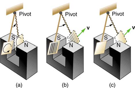
significant drag, called magnetic damping, on the motion involved. Consider the apparatus shown in Figure 23.13, which swings a pendulum bob between the poles of a strong magnet. (This is another favorite physics lab activity.) If the bob is metal, there is significant drag on the bob as it enters
and leaves the field, quickly damping the motion. If, however, the bob is a slotted metal plate, as shown in Figure 23.13(b), there is a much smaller effect due to the magnet. There is no discernible effect on a bob made of an insulator. Why is there drag in both directions, and are there any uses for
magnetic drag?
Figure 23.13 A common physics demonstration device for exploring eddy currents and magnetic damping. (a) The motion of a metal pendulum bob swinging between the
poles of a magnet is quickly damped by the action of eddy currents. (b) There is little effect on the motion of a slotted metal bob, implying that eddy currents are made less
effective. (c) There is also no magnetic damping on a nonconducting bob, since the eddy currents are extremely small.
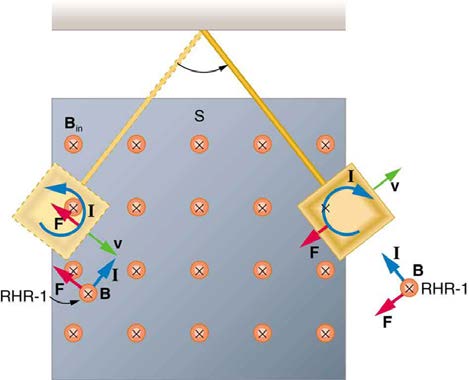
Figure 23.14 shows what happens to the metal plate as it enters and leaves the magnetic field. In both cases, it experiences a force opposing its
motion. As it enters from the left, flux increases, and so an eddy current is set up (Faraday’s law) in the counterclockwise direction (Lenz’s law), as
shown. Only the right-hand side of the current loop is in the field, so that there is an unopposed force on it to the left (RHR-1). When the metal plate is
completely inside the field, there is no eddy current if the field is uniform, since the flux remains constant in this region. But when the plate leaves the
field on the right, flux decreases, causing an eddy current in the clockwise direction that, again, experiences a force to the left, further slowing the
motion. A similar analysis of what happens when the plate swings from the right toward the left shows that its motion is also damped when entering
and leaving the field.
Figure 23.14 A more detailed look at the conducting plate passing between the poles of a magnet. As it enters and leaves the field, the change in flux produces an eddy
current. Magnetic force on the current loop opposes the motion. There is no current and no magnetic drag when the plate is completely inside the uniform field.
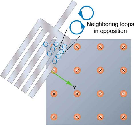
When a slotted metal plate enters the field, as shown in Figure 23.15, an emf is induced by the change in flux, but it is less effective because the slots limit the size of the current loops. Moreover, adjacent loops have currents in opposite directions, and their effects cancel. When an insulating
material is used, the eddy current is extremely small, and so magnetic damping on insulators is negligible. If eddy currents are to be avoided in
conductors, then they can be slotted or constructed of thin layers of conducting material separated by insulating sheets.
CHAPTER 23 | ELECTROMAGNETIC INDUCTION, AC CIRCUITS, AND ELECTRICAL TECHNOLOGIES 823
Figure 23.15 Eddy currents induced in a slotted metal plate entering a magnetic field form small loops, and the forces on them tend to cancel, thereby making magnetic drag
almost zero.
Applications of Magnetic Damping
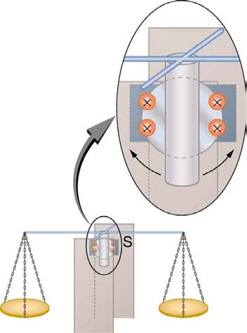
One use of magnetic damping is found in sensitive laboratory balances. To have maximum sensitivity and accuracy, the balance must be as friction-
free as possible. But if it is friction-free, then it will oscillate for a very long time. Magnetic damping is a simple and ideal solution. With magnetic
damping, drag is proportional to speed and becomes zero at zero velocity. Thus the oscillations are quickly damped, after which the damping force
disappears, allowing the balance to be very sensitive. (See Figure 23.16.) In most balances, magnetic damping is accomplished with a conducting
disc that rotates in a fixed field.
Figure 23.16 Magnetic damping of this sensitive balance slows its oscillations. Since Faraday’s law of induction gives the greatest effect for the most rapid change, damping is greatest for large oscillations and goes to zero as the motion stops.
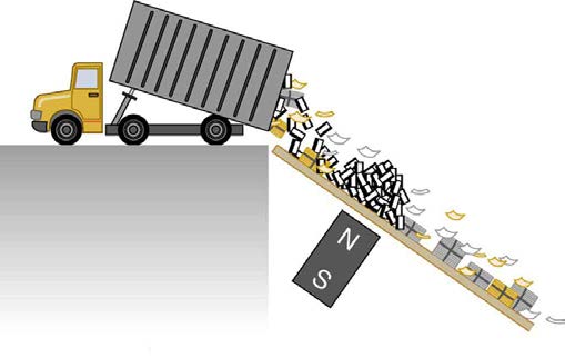
Since eddy currents and magnetic damping occur only in conductors, recycling centers can use magnets to separate metals from other materials.
Trash is dumped in batches down a ramp, beneath which lies a powerful magnet. Conductors in the trash are slowed by magnetic damping while
nonmetals in the trash move on, separating from the metals. (See Figure 23.17.) This works for all metals, not just ferromagnetic ones. A magnet can
separate out the ferromagnetic materials alone by acting on stationary trash.

824 CHAPTER 23 | ELECTROMAGNETIC INDUCTION, AC CIRCUITS, AND ELECTRICAL TECHNOLOGIES
Figure 23.17 Metals can be separated from other trash by magnetic drag. Eddy currents and magnetic drag are created in the metals sent down this ramp by the powerful
magnet beneath it. Nonmetals move on.
Other major applications of eddy currents are in metal detectors and braking systems in trains and roller coasters. Portable metal detectors (Figure
23.18) consist of a primary coil carrying an alternating current and a secondary coil in which a current is induced. An eddy current will be induced in a piece of metal close to the detector which will cause a change in the induced current within the secondary coil, leading to some sort of signal like a
shrill noise. Braking using eddy currents is safer because factors such as rain do not affect the braking and the braking is smoother. However, eddy
currents cannot bring the motion to a complete stop, since the force produced decreases with speed. Thus, speed can be reduced from say 20 m/s to
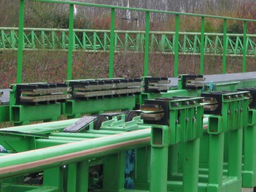
5 m/s, but another form of braking is needed to completely stop the vehicle. Generally, powerful rare earth magnets such as neodymium magnets are
used in roller coasters. Figure 23.19 shows rows of magnets in such an application. The vehicle has metal fins (normally containing copper) which
pass through the magnetic field slowing the vehicle down in much the same way as with the pendulum bob shown in Figure 23.13.
Figure 23.18 A soldier in Iraq uses a metal detector to search for explosives and weapons. (credit: U.S. Army)
Figure 23.19 The rows of rare earth magnets (protruding horizontally) are used for magnetic braking in roller coasters. (credit: Stefan Scheer, Wikimedia Commons)
Induction cooktops have electromagnets under their surface. The magnetic field is varied rapidly producing eddy currents in the base of the pot,
causing the pot and its contents to increase in temperature. Induction cooktops have high efficiencies and good response times but the base of the
pot needs to be ferromagnetic, iron or steel for induction to work.
CHAPTER 23 | ELECTROMAGNETIC INDUCTION, AC CIRCUITS, AND ELECTRICAL TECHNOLOGIES 825
23.5 Electric Generators
Electric generators induce an emf by rotating a coil in a magnetic field, as briefly discussed in Induced Emf and Magnetic Flux. We will now explore generators in more detail. Consider the following example.
Example 23.3 Calculating the Emf Induced in a Generator Coil
The generator coil shown in Figure 23.20 is rotated through one-fourth of a revolution (from θ = 0º to θ = 90º ) in 15.0 ms. The 200-turn circular coil has a 5.00 cm radius and is in a uniform 1.25 T magnetic field. What is the average emf induced?
Figure 23.20 When this generator coil is rotated through one-fourth of a revolution, the magnetic flux Φ changes from its maximum to zero, inducing an emf.
Strategy
We use Faraday’s law of induction to find the average emf induced over a time Δ t :
(23.11)
emf = − NΔ Φ
Δ t .
We know that N = 200 and Δ t = 15.0 ms , and so we must determine the change in flux Δ Φ to find emf.
Solution
Since the area of the loop and the magnetic field strength are constant, we see that
(23.12)
Δ Φ = Δ( BA cos θ) = ABΔ(cos θ).
Now, Δ(cos θ) = −1.0 , since it was given that θ goes from 0º to 90º . Thus Δ Φ = − AB , and
(23.13)
emf = N AB
Δ t .
The area of the loop is A = πr 2 = (3.14...)(0.0500 m)2 = 7.85×10⁻³ m2 . Entering this value gives
(23.14)
emf = 200(7.85×10⁻³ m2)(1.25 T) = 131 V.
15.0×10⁻³ s
Discussion
This is a practical average value, similar to the 120 V used in household power.
The emf calculated in Example 23.3 is the average over one-fourth of a revolution. What is the emf at any given instant? It varies with the angle
between the magnetic field and a perpendicular to the coil. We can get an expression for emf as a function of time by considering the motional emf on
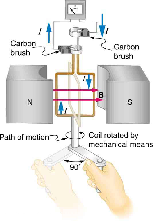
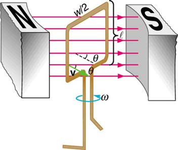
a rotating rectangular coil of width w and height ℓ in a uniform magnetic field, as illustrated in Figure 23.21.
826 CHAPTER 23 | ELECTROMAGNETIC INDUCTION, AC CIRCUITS, AND ELECTRICAL TECHNOLOGIES
Figure 23.21 A generator with a single rectangular coil rotated at constant angular velocity in a uniform magnetic field produces an emf that varies sinusoidally in time. Note
the generator is similar to a motor, except the shaft is rotated to produce a current rather than the other way around.
Charges in the wires of the loop experience the magnetic force, because they are moving in a magnetic field. Charges in the vertical wires experience
forces parallel to the wire, causing currents. But those in the top and bottom segments feel a force perpendicular to the wire, which does not cause a
current. We can thus find the induced emf by considering only the side wires. Motional emf is given to be emf = Bℓv , where the velocity v is
perpendicular to the magnetic field B . Here the velocity is at an angle θ with B , so that its component perpendicular to B is v sin θ (see Figure
23.21). Thus in this case the emf induced on each side is emf = Bℓv sin θ , and they are in the same direction. The total emf around the loop is then
(23.15)
emf = 2 Bℓv sin θ.
This expression is valid, but it does not give emf as a function of time. To find the time dependence of emf, we assume the coil rotates at a constant
angular velocity ω . The angle θ is related to angular velocity by θ = ωt , so that
(23.16)
emf = 2 Bℓv sin ωt.
Now, linear velocity v is related to angular velocity ω by v = rω . Here r = w / 2 , so that v = (w / 2)ω , and
(23.17)
emf = 2 Bℓw 2 ω sin ωt = ( ℓw) Bω sin ωt.
Noting that the area of the loop is A = ℓw , and allowing for N loops, we find that
(23.18)
emf = NABω sin ωt
is the emf induced in a generator coil of N turns and area A rotating at a constant angular velocity ω in a uniform magnetic field B . This can also be expressed as
(23.19)
emf = emf0 sin ωt,
where
(23.20)
emf0 = NABω
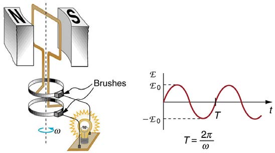
is the maximum (peak) emf. Note that the frequency of the oscillation is f = ω / 2π , and the period is T = 1 / f = 2π / ω . Figure 23.22 shows a graph of emf as a function of time, and it now seems reasonable that AC voltage is sinusoidal.
Figure 23.22 The emf of a generator is sent to a light bulb with the system of rings and brushes shown. The graph gives the emf of the generator as a function of time. emf0
is the peak emf. The period is T = 1 / f = 2π / ω , where f is the frequency. Note that the script E stands for emf.
The fact that the peak emf, emf0 = NABω , makes good sense. The greater the number of coils, the larger their area, and the stronger the field, the
greater the output voltage. It is interesting that the faster the generator is spun (greater ω ), the greater the emf. This is noticeable on bicycle
generators—at least the cheaper varieties. One of the authors as a juvenile found it amusing to ride his bicycle fast enough to burn out his lights, until
he had to ride home lightless one dark night.
CHAPTER 23 | ELECTROMAGNETIC INDUCTION, AC CIRCUITS, AND ELECTRICAL TECHNOLOGIES 827
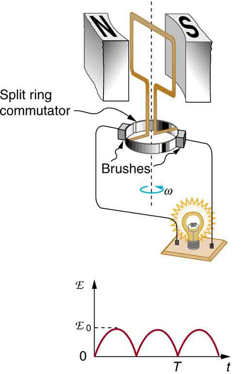
Figure 23.23 shows a scheme by which a generator can be made to produce pulsed DC. More elaborate arrangements of multiple coils and split
rings can produce smoother DC, although electronic rather than mechanical means are usually used to make ripple-free DC.
Figure 23.23 Split rings, called commutators, produce a pulsed DC emf output in this configuration.
Example 23.4 Calculating the Maximum Emf of a Generator
Calculate the maximum emf, emf0 , of the generator that was the subject of Example 23.3.
Strategy
Once ω , the angular velocity, is determined, emf0 = NABω can be used to find emf0 . All other quantities are known.
Solution
Angular velocity is defined to be the change in angle per unit time:
(23.21)
ω = Δ θ
Δ t .
One-fourth of a revolution is π/2 radians, and the time is 0.0150 s; thus,
(23.22)
ω = π / 2 rad
0.0150 s
= 1047 rad/s.
104.7 rad/s is exactly 1000 rpm. We substitute this value for ω and the information from the previous example into emf0 = NABω , yielding
(23.23)
emf0 = NABω
= 200(7.85×10⁻³ m2)(1.25 T)(104.7 rad/s).
= 206 V
Discussion
The maximum emf is greater than the average emf of 131 V found in the previous example, as it should be.
In real life, electric generators look a lot different than the figures in this section, but the principles are the same. The source of mechanical energy
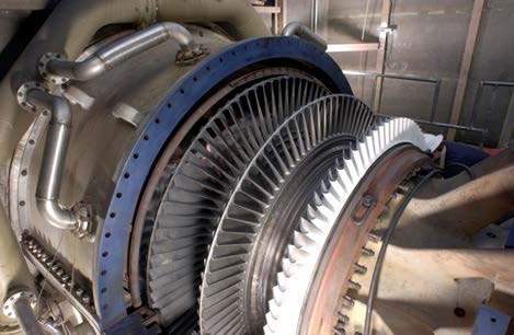
that turns the coil can be falling water (hydropower), steam produced by the burning of fossil fuels, or the kinetic energy of wind. Figure 23.24 shows a cutaway view of a steam turbine; steam moves over the blades connected to the shaft, which rotates the coil within the generator.
828 CHAPTER 23 | ELECTROMAGNETIC INDUCTION, AC CIRCUITS, AND ELECTRICAL TECHNOLOGIES
Figure 23.24 Steam turbine/generator. The steam produced by burning coal impacts the turbine blades, turning the shaft which is connected to the generator. (credit:
Nabonaco, Wikimedia Commons)
Generators illustrated in this section look very much like the motors illustrated previously. This is not coincidental. In fact, a motor becomes a
generator when its shaft rotates. Certain early automobiles used their starter motor as a generator. In Back Emf, we shall further explore the action of a motor as a generator.
23.6 Back Emf
It has been noted that motors and generators are very similar. Generators convert mechanical energy into electrical energy, whereas motors convert
electrical energy into mechanical energy. Furthermore, motors and generators have the same construction. When the coil of a motor is turned,
magnetic flux changes, and an emf (consistent with Faraday’s law of induction) is induced. The motor thus acts as a generator whenever its coil
rotates. This will happen whether the shaft is turned by an external input, like a belt drive, or by the action of the motor itself. That is, when a motor is
doing work and its shaft is turning, an emf is generated. Lenz’s law tells us the emf opposes any change, so that the input emf that powers the motor
will be opposed by the motor’s self-generated emf, called the back emf of the motor. (See Figure 23.25.)
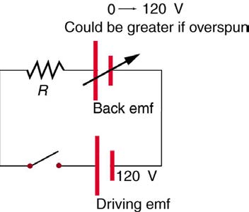
Figure 23.25 The coil of a DC motor is represented as a resistor in this schematic. The back emf is represented as a variable emf that opposes the one driving the motor. Back
emf is zero when the motor is not turning, and it increases proportionally to the motor’s angular velocity.
Back emf is the generator output of a motor, and so it is proportional to the motor’s angular velocity ω . It is zero when the motor is first turned on,
meaning that the coil receives the full driving voltage and the motor draws maximum current when it is on but not turning. As the motor turns faster
and faster, the back emf grows, always opposing the driving emf, and reduces the voltage across the coil and
Describe what you're looking for in as much detail as you'd like.
Our AI reads your request and finds the best matching books for you.
Popular searches:
Join 2.9 million readers and get unlimited free ebooks