College Physics (2012) by Manjula Sharma, Paul Peter Urone, et al - HTML preview
Download the book in PDF, ePub, Kindle for a complete version.
In the previous section, we explored the relationship between voltage and energy. In this section, we will explore the relationship between voltage and
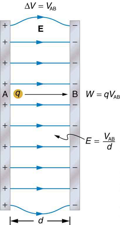
electric field. For example, a uniform electric field E is produced by placing a potential difference (or voltage) Δ V across two parallel metal plates,
labeled A and B. (See Figure 19.5.) Examining this will tell us what voltage is needed to produce a certain electric field strength; it will also reveal a
more fundamental relationship between electric potential and electric field. From a physicist’s point of view, either Δ V or E can be used to describe
any charge distribution. Δ V is most closely tied to energy, whereas E is most closely related to force. Δ V is a scalar quantity and has no
direction, while E is a vector quantity, having both magnitude and direction. (Note that the magnitude of the electric field strength, a scalar quantity,
is represented by E below.) The relationship between Δ V and E is revealed by calculating the work done by the force in moving a charge from
point A to point B. But, as noted in Electric Potential Energy: Potential Difference, this is complex for arbitrary charge distributions, requiring
calculus. We therefore look at a uniform electric field as an interesting special case.
CHAPTER 19 | ELECTRIC POTENTIAL AND ELECTRIC FIELD 669
Figure 19.5 The relationship between V and E for parallel conducting plates is E = V / d . (Note that Δ V = V AB in magnitude. For a charge that is moved from plate A at higher potential to plate B at lower potential, a minus sign needs to be included as follows: –Δ V = V A – V B = V AB . See the text for details.) The work done by the electric field in Figure 19.5 to move a positive charge q from A, the positive plate, higher potential, to B, the negative plate, lower potential, is
W
(19.21)
= –ΔPE = – qΔ V.
The potential difference between points A and B is
(19.22)
–Δ V = – ( V B – V A) = V A – V B = V AB.
Entering this into the expression for work yields
W
(19.23)
= qV AB.
Work is W = Fd cos θ ; here cos θ = 1 , since the path is parallel to the field, and so W = Fd . Since F = qE , we see that W = qEd .
Substituting this expression for work into the previous equation gives
qEd
(19.24)
= qV AB.
The charge cancels, and so the voltage between points A and B is seen to be
V
(19.25)
AB = Ed⎫
⎬(uniform E - field only),
E = V AB
d ⎭
where d is the distance from A to B, or the distance between the plates in Figure 19.5. Note that the above equation implies the units for electric
field are volts per meter. We already know the units for electric field are newtons per coulomb; thus the following relation among units is valid:
(19.26)
1 N / C = 1 V / m.
Voltage between Points A and B
V
(19.27)
AB = Ed⎫
⎬(uniform E - field only),
E = V AB
d ⎭
where d is the distance from A to B, or the distance between the plates.
Example 19.4 What Is the Highest Voltage Possible between Two Plates?
Dry air will support a maximum electric field strength of about 3.0 × 10⁶ V/m . Above that value, the field creates enough ionization in the air to
make the air a conductor. This allows a discharge or spark that reduces the field. What, then, is the maximum voltage between two parallel
conducting plates separated by 2.5 cm of dry air?
670 CHAPTER 19 | ELECTRIC POTENTIAL AND ELECTRIC FIELD
Strategy
We are given the maximum electric field E between the plates and the distance d between them. The equation V AB = Ed can thus be used
to calculate the maximum voltage.
Solution
The potential difference or voltage between the plates is
(19.28)
VAB = Ed.
Entering the given values for E and d gives
(19.29)
V AB = (3.0 × 10⁶ V/m)(0.025 m) = 7.5 × 10⁴ V
or
V
(19.30)
AB = 75 kV.
(The answer is quoted to only two digits, since the maximum field strength is approximate.)
Discussion
One of the implications of this result is that it takes about 75 kV to make a spark jump across a 2.5 cm (1 in.) gap, or 150 kV for a 5 cm spark.
This limits the voltages that can exist between conductors, perhaps on a power transmission line. A smaller voltage will cause a spark if there are
points on the surface, since points create greater fields than smooth surfaces. Humid air breaks down at a lower field strength, meaning that a
smaller voltage will make a spark jump through humid air. The largest voltages can be built up, say with static electricity, on dry days.
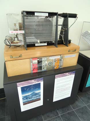
Figure 19.6 A spark chamber is used to trace the paths of high-energy particles. Ionization created by the particles as they pass through the gas between the plates allows a
spark to jump. The sparks are perpendicular to the plates, following electric field lines between them. The potential difference between adjacent plates is not high enough to
cause sparks without the ionization produced by particles from accelerator experiments (or cosmic rays). (credit: Daderot, Wikimedia Commons)
Example 19.5 Field and Force inside an Electron Gun
(a) An electron gun has parallel plates separated by 4.00 cm and gives electrons 25.0 keV of energy. What is the electric field strength between
the plates? (b) What force would this field exert on a piece of plastic with a 0.500 μC charge that gets between the plates?
Strategy
Since the voltage and plate separation are given, the electric field strength can be calculated directly from the expression E = V AB
d . Once the
electric field strength is known, the force on a charge is found using F = q E . Since the electric field is in only one direction, we can write this
equation in terms of the magnitudes, F = q E .
Solution for (a)
The expression for the magnitude of the electric field between two uniform metal plates is
(19.31)
E = V AB
d .
Since the electron is a single charge and is given 25.0 keV of energy, the potential difference must be 25.0 kV. Entering this value for V AB and
the plate separation of 0.0400 m, we obtain
CHAPTER 19 | ELECTRIC POTENTIAL AND ELECTRIC FIELD 671
(19.32)
E = 25.0 kV
0.0400 m = 6.25 × 10⁵ V/m.
Solution for (b)
The magnitude of the force on a charge in an electric field is obtained from the equation
F
(19.33)
= qE.
Substituting known values gives
(19.34)
F = (0.500 × 10⁻⁶ C)(6.25 × 10⁵ V/m) = 0.313 N.
Discussion
Note that the units are newtons, since 1 V/m = 1 N/C . The force on the charge is the same no matter where the charge is located between
the plates. This is because the electric field is uniform between the plates.
In more general situations, regardless of whether the electric field is uniform, it points in the direction of decreasing potential, because the force on a
positive charge is in the direction of E and also in the direction of lower potential V . Furthermore, the magnitude of E equals the rate of decrease
of V with distance. The faster V decreases over distance, the greater the electric field. In equation form, the general relationship between voltage
and electric field is
(19.35)
E = – Δ V
Δ s ,
where Δ s is the distance over which the change in potential, Δ V , takes place. The minus sign tells us that E points in the direction of decreasing
potential. The electric field is said to be the gradient (as in grade or slope) of the electric potential.
Relationship between Voltage and Electric Field
In equation form, the general relationship between voltage and electric field is
(19.36)
E = – Δ V
Δ s ,
where Δ s is the distance over which the change in potential, Δ V , takes place. The minus sign tells us that E points in the direction of
decreasing potential. The electric field is said to be the gradient (as in grade or slope) of the electric potential.
For continually changing potentials, Δ V and Δ s become infinitesimals and differential calculus must be employed to determine the electric field.
19.3 Electrical Potential Due to a Point Charge
Point charges, such as electrons, are among the fundamental building blocks of matter. Furthermore, spherical charge distributions (like on a metal
sphere) create external electric fields exactly like a point charge. The electric potential due to a point charge is, thus, a case we need to consider.
Using calculus to find the work needed to move a test charge q from a large distance away to a distance of r from a point charge Q , and noting
the connection between work and potential ⎛⎝ W = – qΔ V⎞⎠ , it can be shown that the electric potential V of a point charge is
(19.37)
V = kQ
r (Point Charge) ,
where k is a constant equal to 9.0×10⁹ N · m2 /C2 .
Electric Potential V of a Point Charge
The electric potential V of a point charge is given by
(19.38)
V = kQ
r (Point Charge) .
The potential at infinity is chosen to be zero. Thus V for a point charge decreases with distance, whereas E for a point charge decreases with
distance squared:
(19.39)
E = Fq = kQ
r 2 .
Recall that the electric potential V is a scalar and has no direction, whereas the electric field E is a vector. To find the voltage due to a combination
of point charges, you add the individual voltages as numbers. To find the total electric field, you must add the individual fields as vectors, taking
magnitude and direction into account. This is consistent with the fact that V is closely associated with energy, a scalar, whereas E is closely
associated with force, a vector.
672 CHAPTER 19 | ELECTRIC POTENTIAL AND ELECTRIC FIELD
Example 19.6 What Voltage Is Produced by a Small Charge on a Metal Sphere?
Charges in static electricity are typically in the nanocoulomb (nC) to microcoulomb ⎛⎝µC⎞⎠ range. What is the voltage 5.00 cm away from the
center of a 1-cm diameter metal sphere that has a −3.00 nC static charge?
Strategy
As we have discussed in Electric Charge and Electric Field, charge on a metal sphere spreads out uniformly and produces a field like that of a
point charge located at its center. Thus we can find the voltage using the equation V = kQ / r .
Solution
Entering known values into the expression for the potential of a point charge, we obtain
(19.40)
V = kQr
= ⎛
⎛–3.00×10⁻⁹ C⎞
⎝9.00×10⁹ N · m2 / C2⎞⎠⎝ 5.00×10⁻² m ⎠
= –540 V.
Discussion
The negative value for voltage means a positive charge would be attracted from a larger distance, since the potential is lower (more negative)
than at larger distances. Conversely, a negative charge would be repelled, as expected.
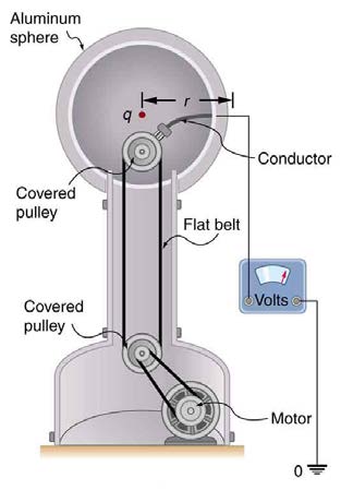
Example 19.7 What Is the Excess Charge on a Van de Graaff Generator
A demonstration Van de Graaff generator has a 25.0 cm diameter metal sphere that produces a voltage of 100 kV near its surface. (See Figure
Figure 19.7 The voltage of this demonstration Van de Graaff generator is measured between the charged sphere and ground. Earth’s potential is taken to be zero as a
reference. The potential of the charged conducting sphere is the same as that of an equal point charge at its center.
Strategy
The potential on the surface will be the same as that of a point charge at the center of the sphere, 12.5 cm away. (The radius of the sphere is
12.5 cm.) We can thus determine the excess charge using the equation
(19.41)
V = kQ
r .
Solution
Solving for Q and entering known values gives
(19.42)
Q = rVk
(0.125 m)⎛
=
⎝100 × 103 V⎞⎠
9.00 × 10⁹ N · m2 / C2
= 1.39 × 10⁻⁶ C = 1.39 µC.
Discussion
CHAPTER 19 | ELECTRIC POTENTIAL AND ELECTRIC FIELD 673
This is a relatively small charge, but it produces a rather large voltage. We have another indication here that it is difficult to store isolated
charges.
The voltages in both of these examples could be measured with a meter that compares the measured potential with ground potential. Ground
potential is often taken to be zero (instead of taking the potential at infinity to be zero). It is the potential difference between two points that is of
importance, and very often there is a tacit assumption that some reference point, such as Earth or a very distant point, is at zero potential. As noted in
Electric Potential Energy: Potential Difference, this is analogous to taking sea level as h = 0 when considering gravitational potential energy, PEg = mgh .
19.4 Equipotential Lines
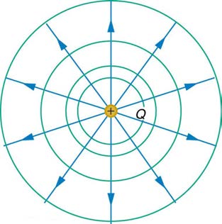
We can represent electric potentials (voltages) pictorially, just as we drew pictures to illustrate electric fields. Of course, the two are related. Consider
Figure 19.8, which shows an isolated positive point charge and its electric field lines. Electric field lines radiate out from a positive charge and terminate on negative charges. While we use blue arrows to represent the magnitude and direction of the electric field, we use green lines to
represent places where the electric potential is constant. These are called equipotential lines in two dimensions, or equipotential surfaces in three
dimensions. The term equipotential is also used as a noun, referring to an equipotential line or surface. The potential for a point charge is the same
anywhere on an imaginary sphere of radius r surrounding the charge. This is true since the potential for a point charge is given by V = kQ / r and,
thus, has the same value at any point that is a given distance r from the charge. An equipotential sphere is a circle in the two-dimensional view of
Figure 19.8. Since the electric field lines point radially away from the charge, they are perpendicular to the equipotential lines.
Figure 19.8 An isolated point charge Q with its electric field lines in blue and equipotential lines in green. The potential is the same along each equipotential line, meaning that no work is required to move a charge anywhere along one of those lines. Work is needed to move a charge from one equipotential line to another. Equipotential lines are
perpendicular to electric field lines in every case.
It is important to note that equipotential lines are always perpendicular to electric field lines. No work is required to move a charge along an
equipotential, since Δ V = 0 . Thus the work is
W
(19.43)
= –ΔPE = – qΔ V = 0.
Work is zero if force is perpendicular to motion. Force is in the same direction as E , so that motion along an equipotential must be perpendicular to
E . More precisely, work is related to the electric field by
W
(19.44)
= Fd cos θ = qEd cos θ = 0.
Note that in the above equation, E and F symbolize the magnitudes of the electric field strength and force, respectively. Neither q nor E nor d is zero, and so cos θ must be 0, meaning θ must be 90º . In other words, motion along an equipotential is perpendicular to E .
One of the rules for static electric fields and conductors is that the electric field must be perpendicular to the surface of any conductor. This implies
that a conductor is an equipotential surface in static situations. There can be no voltage difference across the surface of a conductor, or charges will
flow. One of the uses of this fact is that a conductor can be fixed at zero volts by connecting it to the earth with a good conductor—a process called
grounding. Grounding can be a useful safety tool. For example, grounding the metal case of an electrical appliance ensures that it is at zero volts
relative to the earth.
Grounding
A conductor can be fixed at zero volts by connecting it to the earth with a good conductor—a process called grounding.
Because a conductor is an equipotential, it can replace any equipotential surface. For example, in Figure 19.8 a charged spherical conductor can
replace the point charge, and the electric field and potential surfaces outside of it will be unchanged, confirming the contention that a spherical charge
distribution is equivalent to a point charge at its center.
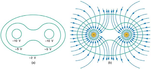
Figure 19.9 shows the electric field and equipotential lines for two equal and opposite charges. Given the electric field lines, the equipotential lines can be drawn simply by making them perpendicular to the electric field lines. Conversely, given the equipotential lines, as in Figure 19.10(a), the electric field lines can be drawn by making them perpendicular to the equipotentials, as in Figure 19.10(b).
674 CHAPTER 19 | ELECTRIC POTENTIAL AND ELECTRIC FIELD
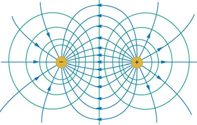
Figure 19.9 The electric field lines and equipotential lines for two equal but opposite charges. The equipotential lines can be drawn by making them perpendicular to the
electric field lines, if those are known. Note that the potential is greatest (most positive) near the positive charge and least (most negative) near the negative charge.
Figure 19.10 (a) These equipotential lines might be measured with a voltmeter in a laboratory experiment. (b) The corresponding electric field lines are found by drawing them
perpendicular to the equipotentials. Note that these fields are consistent with two equal negative charges.
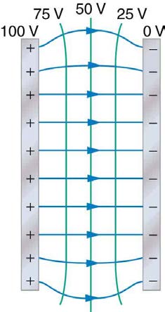
One of the most important cases is that of the familiar parallel conducting plates shown in Figure 19.11. Between the plates, the equipotentials are evenly spaced and parallel. The same field could be maintained by placing conducting plates at the equipotential lines at the potentials shown.
Figure 19.11 The electric field and equipotential lines between two metal plates.
An important application of electric fields and equipotential lines involves the heart. The heart relies on electrical signals to maintain its rhythm. The
movement of electrical signals causes the chambers of the heart to contract and relax. When a person has a heart attack, the movement of these
electrical signals may be disturbed. An artificial pacemaker and a defibrillator can be used to initiate the rhythm of electrical signals. The equipotential
lines around the heart, the thoracic region, and the axis of the heart are useful ways of monitoring the structure and functions of the heart. An
electrocardiogram (ECG) measures the small electric signals being generated during the activity of the heart. More about the relationship between
electric fields and the heart is discussed in Energy Stored in Capacitors.
PhET Explorations: Charges and Fields
Move point charges around on the playing field and then view the electric field, voltages, equipotential lines, and more. It's colorful, it's dynamic,
it's free.

CHAPTER 19 | ELECTRIC POTENTIAL AND ELECTRIC FIELD 675
Figure 19.12 Charges and Fields (http://cnx.org/content/m42331/1.3/charges-and-fields_en.jar)
19.5 Capacitors and Dielectrics
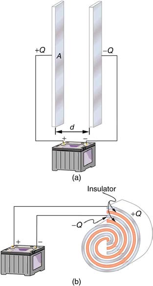
A capacitor is a device used to store electric charge. Capacitors have applications ranging from filtering static out of radio reception to energy
storage in heart defibrillators. Typically, commercial capacitors have two conducting parts close to one another, but not touching, such as those in
Figure 19.13. (Most of the time an insulator is used between the two plates to provide separation—see the discussion on dielectrics below.) When
battery terminals are connected to an initially uncharged capacitor, equal amounts of positive and negative charge, + Q and – Q , are separated
into its two plates. The capacitor remains neutral overall, but we refer to it as storing a charge Q in this circumstance.