College Physics (2012) by Manjula Sharma, Paul Peter Urone, et al - HTML preview
Download the book in PDF, ePub, Kindle for a complete version.
Entrainment
People have long put the Bernoulli principle to work by using reduced pressure in high-velocity fluids to move things about. With a higher pressure on
the outside, the high-velocity fluid forces other fluids into the stream. This process is called entrainment. Entrainment devices have been in use since
ancient times, particularly as pumps to raise water small heights, as in draining swamps, fields, or other low-lying areas. Some other devices that use
the concept of entrainment are shown in Figure 12.5.
Figure 12.5 Examples of entrainment devices that use increased fluid speed to create low pressures, which then entrain one fluid into another. (a) A Bunsen burner uses an
adjustable gas nozzle, entraining air for proper combustion. (b) An atomizer uses a squeeze bulb to create a jet of air that entrains drops of perfume. Paint sprayers and
carburetors use very similar techniques to move their respective liquids. (c) A common aspirator uses a high-speed stream of water to create a region of lower pressure.
Aspirators may be used as suction pumps in dental and surgical situations or for draining a flooded basement or producing a reduced pressure in a vessel. (d) The chimney of
a water heater is designed to entrain air into the pipe leading through the ceiling.
Wings and Sails
The airplane wing is a beautiful example of Bernoulli’s principle in action. Figure 12.6(a) shows the characteristic shape of a wing. The wing is tilted
upward at a small angle and the upper surface is longer, causing air to flow faster over it. The pressure on top of the wing is therefore reduced,
creating a net upward force or lift. (Wings can also gain lift by pushing air downward, utilizing the conservation of momentum principle. The deflected
air molecules result in an upward force on the wing — Newton’s third law.) Sails also have the characteristic shape of a wing. (See Figure 12.6(b).) The pressure on the front side of the sail, P front , is lower than the pressure on the back of the sail, P back . This results in a forward force and even
allows you to sail into the wind.
Making Connections: Take-Home Investigation with Two Strips of Paper
For a good illustration of Bernoulli’s principle, make two strips of paper, each about 15 cm long and 4 cm wide. Hold the small end of one strip up
to your lips and let it drape over your finger. Blow across the paper. What happens? Now hold two strips of paper up to your lips, separated by
your fingers. Blow between the strips. What happens?
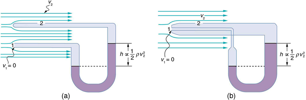
Velocity measurement
Figure 12.7 shows two devices that measure fluid velocity based on Bernoulli’s principle. The manometer in Figure 12.7(a) is connected to two tubes that are small enough not to appreciably disturb the flow. The tube facing the oncoming fluid creates a dead spot having zero velocity ( v 1 = 0 ) in
front of it, while fluid passing the other tube has velocity v
2
2
2 . This means that Bernoulli’s principle as stated in P 1 + 12 ρv 1 = P 2 + 12 ρv 2 becomes
2
(12.26)
P 1 = P 2 + 12 ρv 2.
Figure 12.6 (a) The Bernoulli principle helps explain lift generated by a wing. (b) Sails use the same technique to generate part of their thrust.
404 CHAPTER 12 | FLUID DYNAMICS AND ITS BIOLOGICAL AND MEDICAL APPLICATIONS
Thus pressure P
2
2 over the second opening is reduced by 12 ρv 2 , and so the fluid in the manometer rises by h on the side connected to the second
opening, where
2
(12.27)
h ∝ 12 ρv 2.
(Recall that the symbol ∝ means “proportional to.”) Solving for v 2 , we see that
(12.28)
v 2 ∝ h.
Figure 12.7(b) shows a version of this device that is in common use for measuring various fluid velocities; such devices are frequently used as air speed indicators in aircraft.
Figure 12.7 Measurement of fluid speed based on Bernoulli’s principle. (a) A manometer is connected to two tubes that are close together and small enough not to disturb the
flow. Tube 1 is open at the end facing the flow. A dead spot having zero speed is created there. Tube 2 has an opening on the side, and so the fluid has a speed v across the
1 2
1 2
opening; thus, pressure there drops. The difference in pressure at the manometer is 2 ρv 2 , and so h is proportional to 2 ρv 2 . (b) This type of velocity measuring device is a Prandtl tube, also known as a pitot tube.
12.3 The Most General Applications of Bernoulli’s Equation
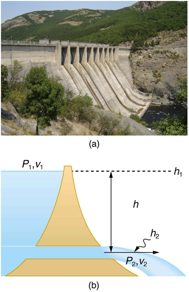
Torricelli’s Theorem
Figure 12.8 shows water gushing from a large tube through a dam. What is its speed as it emerges? Interestingly, if resistance is negligible, the
speed is just what it would be if the water fell a distance h from the surface of the reservoir; the water’s speed is independent of the size of the
opening. Let us check this out. Bernoulli’s equation must be used since the depth is not constant. We consider water flowing from the surface (point
1) to the tube’s outlet (point 2). Bernoulli’s equation as stated in previously is
2
2
(12.29)
P 1 + 12 ρv 1 + ρgh 1 = P 2 + 12 ρv 2 + ρgh 2.
Both P 1 and P 2 equal atmospheric pressure ( P 1 is atmospheric pressure because it is the pressure at the top of the reservoir. P 2 must be
atmospheric pressure, since the emerging water is surrounded by the atmosphere and cannot have a pressure different from atmospheric pressure.)
and subtract out of the equation, leaving
2
2
(12.30)
12 ρv 1+ ρgh 1 = 12 ρv 2+ ρgh 2.
Solving this equation for v 22 , noting that the density ρ cancels (because the fluid is incompressible), yields
2
2
(12.31)
v 2 = v 1 + 2 g( h 1 − h 2).
We let h = h 1 − h 2 ; the equation then becomes
2
2
(12.32)
v 2 = v 1 + 2 gh
where h is the height dropped by the water. This is simply a kinematic equation for any object falling a distance h with negligible resistance. In
fluids, this last equation is called Torricelli’s theorem. Note that the result is independent of the velocity’s direction, just as we found when applying
conservation of energy to falling objects.
CHAPTER 12 | FLUID DYNAMICS AND ITS BIOLOGICAL AND MEDICAL APPLICATIONS 405
Figure 12.8 (a) Water gushes from the base of the Studen Kladenetz dam in Bulgaria. (credit: Kiril Kapustin; http://www.ImagesFromBulgaria.com) (b) In the absence of
significant resistance, water flows from the reservoir with the same speed it would have if it fell the distance h without friction. This is an example of Torricelli’s theorem.
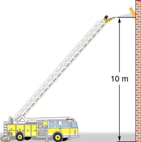
Figure 12.9 Pressure in the nozzle of this fire hose is less than at ground level for two reasons: the water has to go uphill to get to the nozzle, and speed increases in the
nozzle. In spite of its lowered pressure, the water can exert a large force on anything it strikes, by virtue of its kinetic energy. Pressure in the water stream becomes equal to
atmospheric pressure once it emerges into the air.
All preceding applications of Bernoulli’s equation involved simplifying conditions, such as constant height or constant pressure. The next example is a
more general application of Bernoulli’s equation in which pressure, velocity, and height all change. (See Figure 12.9.)
406 CHAPTER 12 | FLUID DYNAMICS AND ITS BIOLOGICAL AND MEDICAL APPLICATIONS
Example 12.5 Calculating Pressure: A Fire Hose Nozzle
Fire hoses used in major structure fires have inside diameters of 6.40 cm. Suppose such a hose carries a flow of 40.0 L/s starting at a gauge
pressure of 1.62×10⁶ N/m2 . The hose goes 10.0 m up a ladder to a nozzle having an inside diameter of 3.00 cm. Assuming negligible
resistance, what is the pressure in the nozzle?
Strategy
Here we must use Bernoulli’s equation to solve for the pressure, since depth is not constant.
Solution
Bernoulli’s equation states
2
2
(12.33)
P 1 + 12 ρv 1 + ρgh 1 = P 2 + 12 ρv 2 + ρgh 2,
where the subscripts 1 and 2 refer to the initial conditions at ground level and the final conditions inside the nozzle, respectively. We must first
find the speeds v 1 and v 2 . Since Q = A 1 v 1 , we get
(12.34)
v 1 = Q
A = 40.0×10⁻³ m3 /s
1
π(3.20×10⁻² m)2 = 12.4 m/s.
Similarly, we find
v
(12.35)
2 = 56.6 m/s.
(This rather large speed is helpful in reaching the fire.) Now, taking h 1 to be zero, we solve Bernoulli’s equation for P 2 :
2
2⎞
(12.36)
P 2 = P 1 + 12 ρ⎛⎝ v 1 − v 2⎠− ρgh 2.
Substituting known values yields
(12.37)
P 2 = 1.62×10⁶ N/m2 + 12(1000 kg/m3)⎡⎣(12.4 m/s)2 − (56.6 m/s)2⎤⎦− (1000 kg/m3)(9.80 m/s2)(10.0 m) = 0.
Discussion
This value is a gauge pressure, since the initial pressure was given as a gauge pressure. Thus the nozzle pressure equals atmospheric
pressure, as it must because the water exits into the atmosphere without changes in its conditions.
Power in Fluid Flow
Power is the rate at which work is done or energy in any form is used or supplied. To see the relationship of power to fluid flow, consider Bernoulli’s
equation:
(12.38)
P + 12 ρv 2 + ρgh = constant.
All three terms have units of energy per unit volume, as discussed in the previous section. Now, considering units, if we multiply energy per unit
volume by flow rate (volume per unit time), we get units of power. That is, ( E / V)( V / t) = E / t . This means that if we multiply Bernoulli’s equation by flow rate Q , we get power. In equation form, this is
⎛
(12.39)
⎝ P + 12 ρv 2 + ρgh⎞⎠ Q = power.
Each term has a clear physical meaning. For example, PQ is the power supplied to a fluid, perhaps by a pump, to give it its pressure P . Similarly,
12 ρv 2 Q is the power supplied to a fluid to give it its kinetic energy. And ρghQ is the power going to gravitational potential energy.
Making Connections: Power
Power is defined as the rate of energy transferred, or E / t . Fluid flow involves several types of power. Each type of power is identified with a
specific type of energy being expended or changed in form.
Example 12.6 Calculating Power in a Moving Fluid
Suppose the fire hose in the previous example is fed by a pump that receives water through a hose with a 6.40-cm diameter coming from a
hydrant with a pressure of 0.700×10⁶ N/m2 . What power does the pump supply to the water?
Strategy
Here we must consider energy forms as well as how they relate to fluid flow. Since the input and output hoses have the same diameters and are
at the same height, the pump does not change the speed of the water nor its height, and so the water’s kinetic energy and gravitational potential
CHAPTER 12 | FLUID DYNAMICS AND ITS BIOLOGICAL AND MEDICAL APPLICATIONS 407
energy are unchanged. That means the pump only supplies power to increase water pressure by 0.92×10⁶ N/m2 (from 0.700×10⁶ N/m2
to 1.62×10⁶ N/m2 ).
Solution
As discussed above, the power associated with pressure is
(12.40)
power = PQ
= ⎛
⎛
⎝0.920×10⁶ N/m2⎞⎠⎝40.0×10−3 m3 /s⎞⎠.
= 3.68×10⁴ W = 36.8 kW
Discussion
Such a substantial amount of power requires a large pump, such as is found on some fire trucks. (This kilowatt value converts to about 50 hp.)
The pump in this example increases only the water’s pressure. If a pump—such as the heart—directly increases velocity and height as well as
pressure, we would have to calculate all three terms to find the power it supplies.
12.4 Viscosity and Laminar Flow; Poiseuille’s Law
Laminar Flow and Viscosity
When you pour yourself a glass of juice, the liquid flows freely and quickly. But when you pour syrup on your pancakes, that liquid flows slowly and
sticks to the pitcher. The difference is fluid friction, both within the fluid itself and between the fluid and its surroundings. We call this property of fluids
viscosity. Juice has low viscosity, whereas syrup has high viscosity. In the previous sections we have considered ideal fluids with little or no viscosity.
In this section, we will investigate what factors, including viscosity, affect the rate of fluid flow.
The precise definition of viscosity is based on laminar, or nonturbulent, flow. Before we can define viscosity, then, we need to define laminar flow and
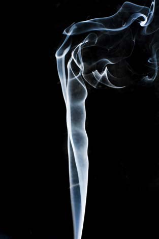
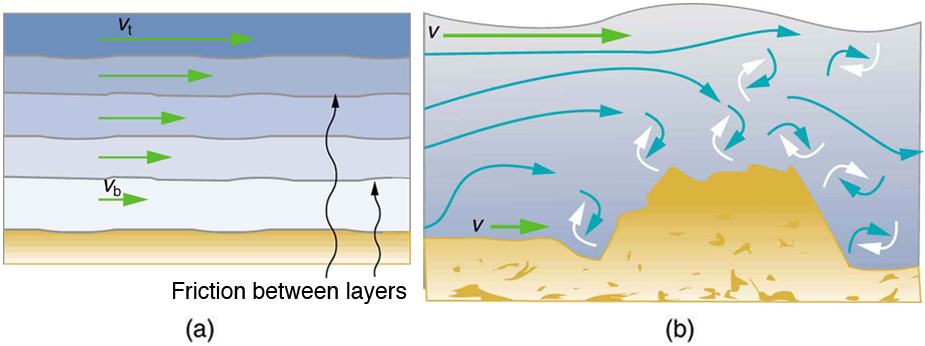
turbulent flow. Figure 12.10 shows both types of flow. Laminar flow is characterized by the smooth flow of the fluid in layers that do not mix.
Turbulent flow, or turbulence, is characterized by eddies and swirls that mix layers of fluid together.
Figure 12.10 Smoke rises smoothly for a while and then begins to form swirls and eddies. The smooth flow is called laminar flow, whereas the swirls and eddies typify
turbulent flow. If you watch the smoke (being careful not to breathe on it), you will notice that it rises more rapidly when flowing smoothly than after it becomes turbulent,
implying that turbulence poses more resistance to flow. (credit: Creativity103)
Figure 12.11 shows schematically how laminar and turbulent flow differ. Layers flow without mixing when flow is laminar. When there is turbulence,
the layers mix, and there are significant velocities in directions other than the overall direction of flow. The lines that are shown in many illustrations
are the paths followed by small volumes of fluids. These are called streamlines. Streamlines are smooth and continuous when flow is laminar, but
break up and mix when flow is turbulent. Turbulence has two main causes. First, any obstruction or sharp corner, such as in a faucet, creates
turbulence by imparting velocities perpendicular to the flow. Second, high speeds cause turbulence. The drag both between adjacent layers of fluid
and between the fluid and its surroundings forms swirls and eddies, if the speed is great enough. We shall concentrate on laminar flow for the
remainder of this section, leaving certain aspects of turbulence for later sections.
408 CHAPTER 12 | FLUID DYNAMICS AND ITS BIOLOGICAL AND MEDICAL APPLICATIONS
Figure 12.11 (a) Laminar flow occurs in layers without mixing. Notice that viscosity causes drag between layers as well as with the fixed surface. (b) An obstruction in the
vessel produces turbulence. Turbulent flow mixes the fluid. There is more interaction, greater heating, and more resistance than in laminar flow.
Making Connections: Take-Home Experiment: Go Down to the River
Try dropping simultaneously two sticks into a flowing river, one near the edge of the river and one near the middle. Which one travels faster?
Why?
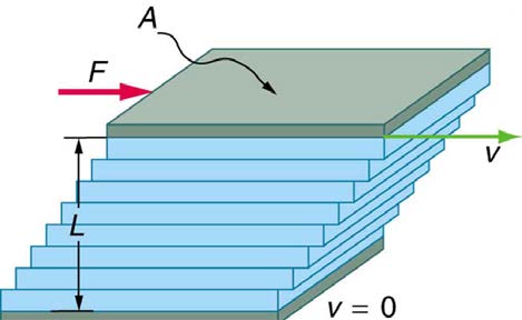
Figure 12.12 shows how viscosity is measured for a fluid. Two parallel plates have the specific fluid between them. The bottom plate is held fixed, while the top plate is moved to the right, dragging fluid with it. The layer (or lamina) of fluid in contact with either plate does not move relative to the
plate, and so the top layer moves at v while the bottom layer remains at rest. Each successive layer from the top down exerts a force on the one
below it, trying to drag it along, producing a continuous variation in speed from v to 0 as shown. Care is taken to insure that the flow is laminar; that
is, the layers do not mix. The motion in Figure 12.12 is like a continuous shearing motion. Fluids have zero shear strength, but the rate at which they are sheared is related to the same geometrical factors A and L as is shear deformation for solids.
Figure 12.12 The graphic shows laminar flow of fluid between two plates of area A . The bottom plate is fixed. When the top plate is pushed to the right, it drags the fluid along with it.
A force F is required to keep the top plate in Figure 12.12 moving at a constant velocity v , and experiments have shown that this force depends on four factors. First, F is directly proportional to v (until the speed is so high that turbulence occurs—then a much larger force is needed, and it has a
more complicated dependence on v ). Second, F is proportional to the area A of the plate. This relationship seems reasonable, since A is directly
proportional to the amount of fluid being moved. Third, F is inversely proportional to the distance between the plates L . This relationship is also
reasonable; L is like a lever arm, and the greater the lever arm, the less force that is needed. Fourth, F is directly proportional to the coefficient of
viscosity, η . The greater the viscosity, the greater the force required. These dependencies are combined into the equation
(12.41)
F = ηvA
L ,
which gives us a working definition of fluid viscosity η . Solving for η gives
(12.42)
η = FL
vA,
which defines viscosity in terms of how it is measured. The SI unit of viscosity is N ⋅ m/[(m/s)m2 ] = (N/m2)s or Pa ⋅ s . Table 12.1 lists the
coefficients of viscosity for various fluids.
Viscosity varies from one fluid to another by several orders of magnitude. As you might expect, the viscosities of gases are much less than those of
liquids, and these viscosities are often temperature dependent. The viscosity of blood can be reduced by aspirin consumption, allowing it to flow more
easily around the body. (When used over the long term in low doses, aspirin can help prevent heart attacks, and reduce the risk of blood clotting.)
Laminar Flow Confined to Tubes—Poiseuille’s Law
What causes flow? The answer, not surprisingly, is pressure difference. In fact, there is a very simple relationship between horizontal flow and
pressure. Flow rate Q is in the direction from high to low pressure. The greater the pressure differential between two points, the greater the flow
rate. This relationship can be stated as
CHAPTER 12 | FLUID DYNAMICS AND ITS BIOLOGICAL AND MEDICAL APPLICATIONS 409
(12.43)
Q = P 2 − P 1
R
,
where P 1 and P 2 are the pressures at two points, such as at either end of a tube, and R is the resistance to flow. The resistance R includes
everything, except pressure, that affects flow rate. For example, R is greater for a long tube than for a short one. The greater the viscosity of a fluid,
the greater the value of R . Turbulence greatly increases R , whereas increasing the diameter of a tube decreases R .
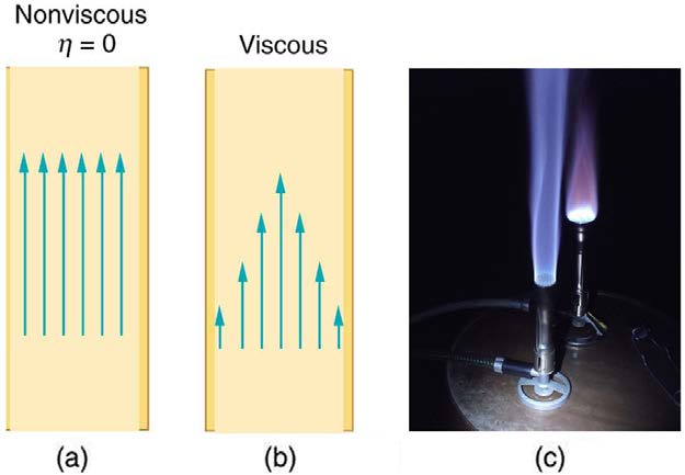
If viscosity is zero, the fluid is frictionless and the resistance to flow is also zero. Comparing frictionless flow in a tube to viscous flow, as in Figure
12.13, we see that for a viscous fluid, speed is greatest at midstream because of drag at the boundaries. We can see the effect of viscosity in a
Bunsen burner flame, even though the viscosity of natural gas is small.
The resistance R to laminar flow of an incompressible fluid having viscosity η through a horizontal tube of uniform radius r and length l , such as
the one in Figure 12.14, is given by
(12.44)
R = 8 ηl
πr 4.
This equation is called Poiseuille’s law for resistance after the French scientist J. L. Poiseuille (1799–1869), who derived it in an attempt to
understand the flow of blood, an often turbulent fluid.
Figure 12.13 (a) If fluid flow in a tube has negligible resistance, the speed is the same all across the tube. (b) When a viscous fluid flows through a tube, its speed at the walls is zero, increasing steadily to its maximum at the center of the tube. (c) The shape of the Bunsen burner flame is due to the velocity profile across the tube. (credit: Jason
Woodhead)
Let us examine Poiseuille’s expression for R to see if it makes good intuitive sense. We see that resistance is directly proportional to both fluid
viscosity η and the length l of a tube. After all, both of these directly affect the amount of friction encountered—the greater either is, the greater the
resistance and the smaller the flow. The radius r of a tube affects the resistance, which again makes sense, because the greater the radius, the
greater the flow (all other factors remaining the same). But it is surprising that r is raised to the fourth power in Poiseuille’s law. This exponent
means that any change in the radius of a tube has a very large effect on resistance. For example, doubling the radius of a tube decreases resistance
by a factor of 24 = 16 .
Taken together, Q = P 2 − P 1
R
and R = 8 ηl
πr 4 give the following expression for flow rate:
(12.45)
Q = ( P 2 − P 1) πr 4
8 ηl
.
This equation describes laminar flow through a tube. It is sometimes called Poiseuille’s law for laminar flow, or simply Poiseuille’s law.