College Physics (2012) by Manjula Sharma, Paul Peter Urone, et al - HTML preview
Download the book in PDF, ePub, Kindle for a complete version.
laminar at low velocity. We also know that at high velocity, even flow in a smooth tube or around a smooth object will experience turbulence. In
between, it is more difficult to predict. In fact, at intermediate velocities, flow may oscillate back and forth indefinitely between laminar and turbulent.
An occlusion, or narrowing, of an artery, such as shown in Figure 12.17, is likely to cause turbulence because of the irregularity of the blockage, as
well as the complexity of blood as a fluid. Turbulence in the circulatory system is noisy and can sometimes be detected with a stethoscope, such as
when measuring diastolic pressure in the upper arm’s partially collapsed brachial artery. These turbulent sounds, at the onset of blood flow when the
cuff pressure becomes sufficiently small, are called Korotkoff sounds. Aneurysms, or ballooning of arteries, create significant turbulence and can
sometimes be detected with a stethoscope. Heart murmurs, consistent with their name, are sounds produced by turbulent flow around damaged and
insufficiently closed heart valves. Ultrasound can also be used to detect turbulence as a medical indicator in a process analogous to Doppler-shift
radar used to detect storms.
Figure 12.17 Flow is laminar in the large part of this blood vessel and turbulent in the part narrowed by plaque, where velocity is high. In the transition region, the flow can oscillate chaotically between laminar and turbulent flow.
414 CHAPTER 12 | FLUID DYNAMICS AND ITS BIOLOGICAL AND MEDICAL APPLICATIONS
An indicator called the Reynolds number N R can reveal whether flow is laminar or turbulent. For flow in a tube of uniform diameter, the Reynolds
number is defined as
(12.53)
N R = 2 ρvr
η (flow in tube),
where ρ is the fluid density, v its speed, η its viscosity, and r the tube radius. The Reynolds number is a unitless quantity. Experiments have
revealed that N R is related to the onset of turbulence. For N R below about 2000, flow is laminar. For N R above about 3000, flow is turbulent. For
values of N R between about 2000 and 3000, flow is unstable—that is, it can be laminar, but small obstructions and surface roughness can make it
turbulent, and it may oscillate randomly between being laminar and turbulent. The blood flow through most of the body is a quiet, laminar flow. The
exception is in the aorta, where the speed of the blood flow rises above a critical value of 35 m/s and becomes turbulent.
Example 12.9 Is This Flow Laminar or Turbulent?
Calculate the Reynolds number for flow in the needle considered in Example 12.8 to verify the assumption that the flow is laminar. Assume that
the density of the saline solution is 1025 kg/m3 .
Strategy
We have all of the information needed, except the fluid speed v , which can be calculated from v¯ = Q / A = 1.70 m/s (verification of this is in
this chapter’s Problems and Exercises).
Solution
Entering the known values into N R = 2 ρvr
η gives
(12.54)
N R = 2 ρvr
η
= 2(1025 kg/m3)(1.70 m/s)(0.150×10−3 m)
1.00×10⁻³ N ⋅ s/m2
= 523.
Discussion
Since N R is well below 2000, the flow should indeed be laminar.
Take-Home Experiment: Inhalation
Under the conditions of normal activity, an adult inhales about 1 L of air during each inhalation. With the aid of a watch, determine the time for
one of your own inhalations by timing several breaths and dividing the total length by the number of breaths. Calculate the average flow rate Q
of air traveling through the trachea during each inhalation.
The topic of chaos has become quite popular over the last few decades. A system is defined to be chaotic when its behavior is so sensitive to some
factor that it is extremely difficult to predict. The field of chaos is the study of chaotic behavior. A good example of chaotic behavior is the flow of a
fluid with a Reynolds number between 2000 and 3000. Whether or not the flow is turbulent is difficult, but not impossible, to predict—the difficulty lies
in the extremely sensitive dependence on factors like roughness and obstructions on the nature of the flow. A tiny variation in one factor has an
exaggerated (or nonlinear) effect on the flow. Phenomena as disparate as turbulence, the orbit of Pluto, and the onset of irregular heartbeats are
chaotic and can be analyzed with similar techniques.
12.6 Motion of an Object in a Viscous Fluid
A moving object in a viscous fluid is equivalent to a stationary object in a flowing fluid stream. (For example, when you ride a bicycle at 10 m/s in still
air, you feel the air in your face exactly as if you were stationary in a 10-m/s wind.) Flow of the stationary fluid around a moving object may be
laminar, turbulent, or a combination of the two. Just as with flow in tubes, it is possible to predict when a moving object creates turbulence. We use
another form of the Reynolds number N′R , defined for an object moving in a fluid to be
(12.55)
N′R = ρvL
η (object in fluid),
where L is a characteristic length of the object (a sphere’s diameter, for example), ρ the fluid density, η its viscosity, and v the object’s speed in the fluid. If N′R is less than about 1, flow around the object can be laminar, particularly if the object has a smooth shape. The transition to turbulent
flow occurs for N′R between 1 and about 10, depending on surface roughness and so on. Depending on the surface, there can be a turbulent wake
behind the object with some laminar flow over its surface. For an N′R between 10 and 106 , the flow may be either laminar or turbulent and may
CHAPTER 12 | FLUID DYNAMICS AND ITS BIOLOGICAL AND MEDICAL APPLICATIONS 415
oscillate between the two. For N′R greater than about 106 , the flow is entirely turbulent, even at the surface of the object. (See Figure 12.18.) Laminar flow occurs mostly when the objects in the fluid are small, such as raindrops, pollen, and blood cells in plasma.
Example 12.10 Does a Ball Have a Turbulent Wake?
Calculate the Reynolds number N′R for a ball with a 7.40-cm diameter thrown at 40.0 m/s.
Strategy
We can use N′R = ρvL
η to calculate N′R , since all values in it are either given or can be found in tables of density and viscosity.
Solution
Substituting values into the equation for N′R yields
(12.56)
N′ R = ρvL
η = (1.29 kg/m3)(40.0 m/s)(0.0740 m)
1.81×10⁻⁵ 1.00 Pa ⋅ s
= 2.11×10⁵ .
Discussion
This value is sufficiently high to imply a turbulent wake. Most large objects, such as airplanes and sailboats, create significant turbulence as they
move. As noted before, the Bernoulli principle gives only qualitatively-correct results in such situations.
One of the consequences of viscosity is a resistance force called viscous drag F V that is exerted on a moving object. This force typically depends
on the object’s speed (in contrast with simple friction). Experiments have shown that for laminar flow ( N′R less than about one) viscous drag is
proportional to speed, whereas for N′R between about 10 and 106 , viscous drag is proportional to speed squared. (This relationship is a strong
dependence and is pertinent to bicycle racing, where even a small headwind causes significantly increased drag on the racer. Cyclists take turns
being the leader in the pack for this reason.) For N′R greater than 106 , drag increases dramatically and behaves with greater complexity. For
laminar flow around a sphere, F V is proportional to fluid viscosity η , the object’s characteristic size L , and its speed v . All of which makes
sense—the more viscous the fluid and the larger the object, the more drag we expect. Recall Stoke’s law F S = 6 πrηv . For the special case of a
small sphere of radius R moving slowly in a fluid of viscosity η , the drag force F S is given by
F
(12.57)
S = 6 πRηv.
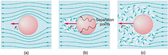
Figure 12.18 (a) Motion of this sphere to the right is equivalent to fluid flow to the left. Here the flow is laminar with N′R less than 1. There is a force, called viscous drag F V , to the left on the ball due to the fluid’s viscosity. (b) At a higher speed, the flow becomes partially turbulent, creating a wake starting where the flow lines separate from the surface. Pressure in the wake is less than in front of the sphere, because fluid speed is less, creating a net force to the left F′V that is significantly greater than for laminar flow. Here N′R is greater than 10. (c) At much higher speeds, where N′R is greater than 106 , flow becomes turbulent everywhere on the surface and behind the
sphere. Drag increases dramatically.
An interesting consequence of the increase in F V with speed is that an object falling through a fluid will not continue to accelerate indefinitely (as it
would if we neglect air resistance, for example). Instead, viscous drag increases, slowing acceleration, until a critical speed, called the terminal
speed, is reached and the acceleration of the object becomes zero. Once this happens, the object continues to fall at constant speed (the terminal
speed). This is the case for particles of sand falling in the ocean, cells falling in a centrifuge, and sky divers falling through the air. Figure 12.19
shows some of the factors that affect terminal speed. There is a viscous drag on the object that depends on the viscosity of the fluid and the size of
the object. But there is also a buoyant force that depends on the density of the object relative to the fluid. Terminal speed will be greatest for low-
viscosity fluids and objects with high densities and small sizes. Thus a skydiver falls more slowly with outspread limbs than when they are in a pike
position—head first with hands at their side and legs together.
416 CHAPTER 12 | FLUID DYNAMICS AND ITS BIOLOGICAL AND MEDICAL APPLICATIONS
Take-Home Experiment: Don’t Lose Your Marbles
By measuring the terminal speed of a slowly moving sphere in a viscous fluid, one can find the viscosity of that fluid (at that temperature). It can
be difficult to find small ball bearings around the house, but a small marble will do. Gather two or three fluids (syrup, motor oil, honey, olive oil,
etc.) and a thick, tall clear glass or vase. Drop the marble into the center of the fluid and time its fall (after letting it drop a little to reach its
terminal speed). Compare your values for the terminal speed and see if they are inversely proportional to the viscosities as listed in Table 12.1.
Does it make a difference if the marble is dropped near the side of the glass?
Knowledge of terminal speed is useful for estimating sedimentation rates of small particles. We know from watching mud settle out of dirty water that
sedimentation is usually a slow process. Centrifuges are used to speed sedimentation by creating accelerated frames in which gravitational
acceleration is replaced by centripetal acceleration, which can be much greater, increasing the terminal speed.
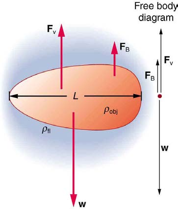
Figure 12.19 There are three forces acting on an object falling through a viscous fluid: its weight w , the viscous drag F V , and the buoyant force FB .
12.7 Molecular Transport Phenomena: Diffusion, Osmosis, and Related Processes
Diffusion
There is something fishy about the ice cube from your freezer—how did it pick up those food odors? How does soaking a sprained ankle in Epsom
salt reduce swelling? The answer to these questions are related to atomic and molecular transport phenomena—another mode of fluid motion. Atoms
and molecules are in constant motion at any temperature. In fluids they move about randomly even in the absence of macroscopic flow. This motion
is called a random walk and is illustrated in Figure 12.20. Diffusion is the movement of substances due to random thermal molecular motion. Fluids, like fish fumes or odors entering ice cubes, can even diffuse through solids.
Diffusion is a slow process over macroscopic distances. The densities of common materials are great enough that molecules cannot travel very far
before having a collision that can scatter them in any direction, including straight backward. It can be shown that the average distance x rms that a
molecule travels is proportional to the square root of time:
(12.58)
x rms = 2 Dt,
where x rms stands for the root-mean-square distance and is the statistical average for the process. The quantity D is the diffusion constant for
the particular molecule in a specific medium. Table 12.2 lists representative values of D for various substances, in units of m2 /s .
CHAPTER 12 | FLUID DYNAMICS AND ITS BIOLOGICAL AND MEDICAL APPLICATIONS 417
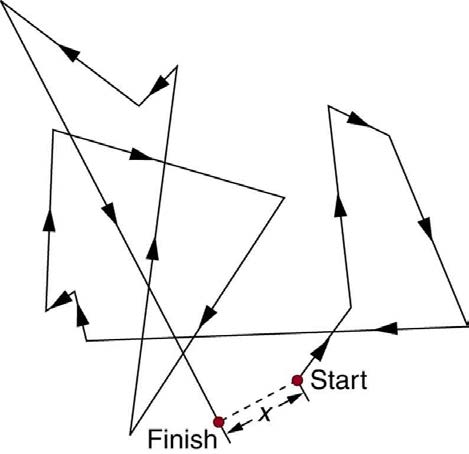
Figure 12.20 The random thermal motion of a molecule in a fluid in time t . This type of motion is called a random walk.
Table 12.2 Diffusion Constants for Various
Molecules[3]
Diffusing molecule
Medium
D (m2/s)
Hydrogen ⎛
⎞
⎝H2⎠
Air
6.4×10⁻⁵
Oxygen ⎛
⎞
⎝O2⎠
Air
1.8×10⁻⁵
Oxygen ⎛
⎞
⎝O2⎠
Water
1.0×10⁻⁹
Glucose ⎛
⎞
⎝C6 H12 O6⎠ Water
6.7×10⁻¹⁰
Hemoglobin
Water
6.9×10⁻¹¹
DNA
Water
1.3×10⁻¹²
Note that D gets progressively smaller for more massive molecules. This decrease is because the average molecular speed at a given temperature
is inversely proportional to molecular mass. Thus the more massive molecules diffuse more slowly. Another interesting point is that D for oxygen in
air is much greater than D for oxygen in water. In water, an oxygen molecule makes many more collisions in its random walk and is slowed
considerably. In water, an oxygen molecule moves only about 40 µ m in 1 s. (Each molecule actually collides about 1010 times per second!).
Finally, note that diffusion constants increase with temperature, because average molecular speed increases with temperature. This is because the
average kinetic energy of molecules, 1
2 mv 2 , is proportional to absolute temperature.
Example 12.11 Calculating Diffusion: How Long Does Glucose Diffusion Take?
Calculate the average time it takes a glucose molecule to move 1.0 cm in water.
Strategy
We can use x rms = 2 Dt , the expression for the average distance moved in time t , and solve it for t . All other quantities are known.
Solution
Solving for t and substituting known values yields
2
(12.59)
t = x rms
2 D =
(0.010 m)2
2(6.7×10⁻¹⁰ m2 /s)
= 7.5×10⁴ s = 21 h.
Discussion
3. At 20°C and 1 atm
418 CHAPTER 12 | FLUID DYNAMICS AND ITS BIOLOGICAL AND MEDICAL APPLICATIONS
This is a remarkably long time for glucose to move a mere centimeter! For this reason, we stir sugar into water rather than waiting for it to diffuse.
Because diffusion is typically very slow, its most important effects occur over small distances. For example, the cornea of the eye gets most of its
oxygen by diffusion through the thin tear layer covering it.
The Rate and Direction of Diffusion
If you very carefully place a drop of food coloring in a still glass of water, it will slowly diffuse into the colorless surroundings until its concentration is
the same everywhere. This type of diffusion is called free diffusion, because there are no barriers inhibiting it. Let us examine its direction and rate.
Molecular motion is random in direction, and so simple chance dictates that more molecules will move out of a region of high concentration than into
it. The net rate of diffusion is higher initially than after the process is partially completed. (See Figure 12.21.)
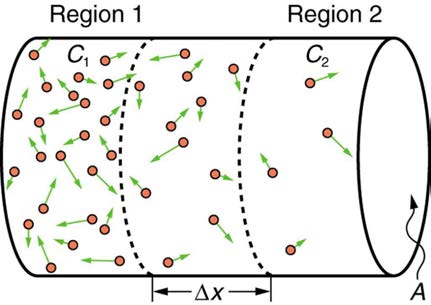
Figure 12.21 Diffusion proceeds from a region of higher concentration to a lower one. The net rate of movement is proportional to the difference in concentration.
The rate of diffusion is proportional to the concentration difference. Many more molecules will leave a region of high concentration than will enter it
from a region of low concentration. In fact, if the concentrations were the same, there would be no net movement. The rate of diffusion is also
proportional to the diffusion constant D , which is determined experimentally. The farther a molecule can diffuse in a given time, the more likely it is to
leave the region of high concentration. Many of the factors that affect the rate are hidden in the diffusion constant D . For example, temperature and
cohesive and adhesive forces all affect values of D .
Diffusion is the dominant mechanism by which the exchange of nutrients and waste products occur between the blood and tissue, and between air
and blood in the lungs. In the evolutionary process, as organisms became larger, they needed quicker methods of transportation than net diffusion,
because of the larger distances involved in the transport, leading to the development of circulatory systems. Less sophisticated, single-celled
organisms still rely totally on diffusion for the removal of waste products and the uptake of nutrients.
Osmosis and Dialysis—Diffusion across Membranes
Some of the most interesting examples of diffusion occur through barriers that affect the rates of diffusion. For example, when you soak a swollen
ankle in Epsom salt, water diffuses through your skin. Many substances regularly move through cell membranes; oxygen moves in, carbon dioxide
moves out, nutrients go in, and wastes go out, for example. Because membranes are thin structures (typically 6.5×10⁻⁹ to 10×10−9 m across)
diffusion rates through them can be high. Diffusion through membranes is an important method of transport.
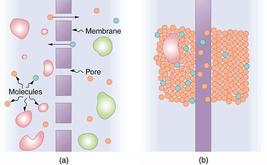
Membranes are generally selectively permeable, or semipermeable. (See Figure 12.22.) One type of semipermeable membrane has small pores
that allow only small molecules to pass through. In other types of membranes, the molecules may actually dissolve in the membrane or react with
molecules in the membrane while moving across. Membrane function, in fact, is the subject of much current research, involving not only physiology
but also chemistry and physics.
Figure 12.22 (a) A semipermeable membrane with small pores that allow only small molecules to pass through. (b) Certain molecules dissolve in this membrane and diffuse
across it.
CHAPTER 12 | FLUID DYNAMICS AND ITS BIOLOGICAL AND MEDICAL APPLICATIONS 419
Osmosis is the transport of water through a semipermeable membrane from a region of high concentration to a region of low concentration. Osmosis
is driven by the imbalance in water concentration. For example, water is more concentrated in your body than in Epsom salt. When you soak a
swollen ankle in Epsom salt, the water moves out of your body into the lower-concentration region in the salt. Similarly, dialysis is the transport of
any other molecule through a semipermeable membrane due to its concentration difference. Both osmosis and dialysis are used by the kidneys to
cleanse the blood.
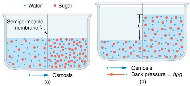
Osmosis can create a substantial pressure. Consider what happens if osmosis continues for some time, as illustrated in Figure 12.23. Water moves
by osmosis from the left into the region on the right, where it is less concentrated, causing the solution on the right to rise. This movement will
continue until the pressure ρgh created by the extra height of fluid on the right is large enough to stop further osmosis. This pressure is called a
back pressure. The back pressure ρgh that stops osmosis is also called the relative osmotic pressure if neither solution is pure water, and it is
called the osmotic pressure if one solution is pure water. Osmotic pressure can be large, depending on the size of the concentration difference. For
example, if pure water and sea water are separated by a semipermeable membrane that passes no salt, osmotic pressure will be 25.9 atm. This
value means that water will diffuse through the membrane until the salt water surface rises 268 m above the pure-water surface! One example of
pressure created by osmosis is turgor in plants (many wilt when too dry). Turgor describes the condition of a plant in which the fluid in a cell exerts a
pressure against the cell wall. This pressure gives the plant support. Dialysis can similarly cause substantial pressures.
Figure 12.23 (a) Two sugar-water solutions of different concentrations, separated by a semipermeable membrane that passes water but not sugar. Osmosis will be to the right,
since water is less concentrated there. (b) The fluid level rises until the back pressure ρgh equals the relative osmotic pressure; then, the net transfer of water is zero.
Reverse osmosis and reverse dialysis (also called filtration) are processes that occur when back pressure is sufficient to reverse the normal
direction of substances through membranes. Back pressure can be created naturally as on the right side of Figure 12.23. (A piston can also create
this pressure.) Reverse osmosis can be used to desalinate water by simply forcing it through a membrane that will not pass salt. Similarly, reverse
dialysis can be used to filter out any substance that a given membrane will not pass.
One further example of the movement of substances through membranes deserves mention. We sometimes find that substances pass in the
direction opposite to what we expect. Cypress tree roots, for example, extract pure water from salt water, although osmosis would move it in the
opposite direction. This is not reverse osmosis, because there is no back pressure to cause it. What is happening is called active transport, a
process in which a living membrane expends energy to move substances across it. Many living membranes move water and other substances by
active transport. The kidneys, for example, not only use osmosis and dialysis—they also employ significant active transport to move substances into
and out of blood. In fact, it is estimated that at least 25% of the body’s energy is expended on active transport of substances at the cellular level. The
study of active transport carries us into the realms of microbiology, biophysics, and biochemistry and it is a fascinating application of the laws of
nature to living structures.
Glossary
active transport: the process in which a living membrane expends energy to move substances across
Bernoulli’s equation: the equation resulting from applying conservation of energy to an incompressible frictionless fluid: P + 1/2