

Classical Electrodynamics by Konstantin K. Likharev - HTML preview
Download the book in PDF, ePub, Kindle for a complete version.
(2.111)
In this case, both functions R and F may be labeled with the integer index n. Taking into account that the terms with negative values of n may be summed up with those with positive n, and that s 0 has to equal zero (otherwise the 2-periodicity of function F would be violated), we see that the general solution of the 2D Laplace equation for such geometries may be represented as
Variable
separation
n
b
in polar
(,) a b ln
a
n
cos
sin
.
(2.112)
0
0
n
c
n s
n
n
n
n
coordinates
n 1
Let us see how all this machinery works on the famous problem of a round cylindrical conductor placed into an electric field that is uniform and perpendicular to the cylinder’s axis at large distances (see Fig. 15a), as if it is created by a large plane capacitor. First of all, let us explore the effect of the system’s symmetries on the coefficients in Eq. (112). Selecting the coordinate system as shown in Fig.
15a, and taking the cylinder’s potential for zero, we immediately get a 0 = 0.
(a)
(b)
E
0
y
R
0
x
Fig. 2.15. A conducting cylinder inserted into an initially uniform electric field perpendicular to its axis: (a) the problem’s geometry, and (b) the equipotential surfaces given by Eq. (117).
Chapter 2
Page 29 of 68
EM: Classical Electrodynamics
Moreover, due to the mirror symmetry about the plane [ x, z], the solution has to be an even function of the angle , and hence all coefficients sn should also equal zero. Also, at large distances (
>> R) from the cylinder, its effect on the electric field should vanish, and the potential should approach that of the uniform external field E = E 0n x:
E x E cos,
for .
(2.113)
0
0
This is only possible if in Eq. (112), b 0 = 0, and also all coefficients an with n 1 vanish, while the product a 1 c 1 should be equal to (– E 0). Thus the solution is reduced to the following form B
(,) E cos
n
cos n ,
(2.114)
0
n
n 1
in which the coefficients Bn bncn should be found from the boundary condition at = R:
( R,) 0 .
(2.115)
This requirement yields the following equation,
B
B
1
E R
cos n cos
n ,
0
(2.116)
0
R
n
n2 R
which should be satisfied for all . This equality, read backward, may be considered as an expansion of a function identically equal to zero into a series over mutually orthogonal functions cos n. It is evidently valid if all coefficients of the expansion, including (– E 0 R + B 1/ R), and all Bn for n 2 are equal to zero. Moreover, mathematics tells us that such expansions are unique, so this is the only possible solution of Eq. (116). So, B 1 = E 0 R 2, and our final answer (valid only outside of the cylinder, i.e. for R), is
R 2
R 2
(,) E
cos E 1
x .
(2.117)
0
0
x 2 y 2
This result, which may be graphically represented with the equipotential surfaces shown in Fig.
15b, shows a smooth transition between the uniform field (113) far from the cylinder, to the equipotential surface of the cylinder (with = 0). Such smoothening is very typical for Laplace equation solutions. Indeed, as we know from Chapter 1, these solutions correspond to the lowest integral of the potential gradient’s square, i.e. to the lowest potential energy (1.65) possible at the given boundary conditions.
To complete the problem, let us use Eq. (3) to calculate the distribution of the surface charge density over the cylinder’s cross-section:
2
R
E
E cos
2
cos.
(2.118)
0
n surface
0
E
0
0
0
0
R
R
This very simple formula shows that with the field direction shown in Fig. 15a ( E 0 > 0), the surface charge is positive on the right-hand side of the cylinder and negative on its left-hand side, thus creating a field directed from the right to the left, which exactly compensates the external field inside the conductor, where the net field is zero. (Please take one more look at the schematic Fig. 1a.) Note also that the net electric charge of the cylinder is zero, in correspondence with the problem symmetry.
Chapter 2
Page 30 of 68


Essential Graduate Physics
EM: Classical Electrodynamics
Another useful by-product of the calculation (118) is that the surface electric field equals 2 E 0cos, and hence its largest magnitude is twice the field far from the cylinder. Such electric field concentration is very typical for all convex conducting surfaces.
The last observation gets additional confirmation from the second possible topology when Eq.
(110) is used to describe problems with no angular periodicity. A typical example of this situation is a cylindrical conductor with a cross-section that features a corner limited by two straight-line segments (Fig. 16). Indeed, we may argue that at < R (where R is the radial extension of the planar sides of the corner, see Fig. 16), the Laplace equation may be satisfied by a sum of partial solutions R() F(), if the angular components of the products satisfy the boundary conditions on the corner sides. Taking (just for the simplicity of notation) the conductor’s potential to be zero, and one of the corner’s sides as the x-
axis ( = 0), these boundary conditions are
F ( )
0 F ( ) 0 ,
(2.119)
where the angle may be anywhere between 0 and 2 – see Fig. 16.
(a)
(b)
R
R
0
Fig. 2.16. The cross-sections
0
of cylindrical conductors with
(a) a corner and (b) a wedge.
Comparing this condition with Eq. (110), we see that it requires s 0 and all c to vanish, and to take one of the values of the following discrete spectrum:
m
,
with m ,
1 ,...
2
.
(2.120)
m
Hence the full solution of the Laplace equation for this geometry takes the form
m/
m
a
sin
,
for R, 0 ,
(2.121)
m
m1
where the constants s have been incorporated into am. The set of coefficients am cannot be universally determined, because it depends on the exact shape of the conductor outside the corner, and the externally applied electric field. However, whatever the set is, in the limit 0, the solution (121) is almost41 always dominated by the term with the lowest m = 1:
/
a
sin ,
(2.122)
1
because the higher terms tend to zero faster. This potential distribution corresponds to the surface charge density
41 Exceptions are possible only for highly symmetric configurations when the external field is specially crafted to make a 1 = 0. In this case, the solution at 0 is dominated by the first nonzero term of the series (121).
Chapter 2
Page 31 of 68
EM: Classical Electrodynamics
a 1 /
1
E
.
(2.123)
0
n surface
0
const, 0
0
()
(It is similar, with the opposite sign, on the opposite face of the angle.)
The result (123) shows that if we are dealing with a concave corner ( < , see Fig. 16a), the charge density (and the surface electric field) tends to zero. On the other hand, at a “convex corner” with
> (actually, a wedge – see Fig. 16b), both the charge and the field’s strength concentrate, formally diverging at 0. (So, do not sit on a roof’s ridge during a thunderstorm; rather hide in a ditch!) We have already seen qualitatively similar effects for the thin round disk and the split plane.
2. 7. Variable separation – cylindrical coordinates
Now, let us discuss how to generalize the approach discussed in the previous section to problems whose geometry is still axially symmetric, but where the electrostatic potential depends not only on the radial and angular coordinates but also on the axial coordinate: / z 0. The classical example of such a problem is shown in Fig. 17. Here the sidewall and the bottom lid of a hollow round cylinder are kept at a fixed potential (say, = 0), but the potential V fixed at the top lid is different. Evidently, this problem is qualitatively similar to the rectangular box problem solved above (Fig. 13), and we will also try to solve it first for the case of arbitrary voltage distribution over the top lid: V = V( , ).
z
V (,)
l
Fig. 2.17. A cylindrical volume
0
R
y
with conducting walls.
x
0
Following the main idea of the variable separation method, let us require that each partial function k in Eq. (84) satisfies the Laplace equation, now in the full cylindrical coordinates { , , z}:42
1
k
1
2
2
k
k 0
.
(2.124)
2
2
2
z
Plugging k in the form of the product R() F()Z( z) into Eq. (124) and then dividing all resulting terms by this product, we get
1
d dR
1
2
d F
1 2
d Z
0
.
(2.125)
2
2
2
R d d F d
Z dz
Since the first two terms of Eq. (125) can only depend on the polar variables and , while the third term, only on z, at least that term should equal a constant. Denoting it (just like we did in the rectangular box problem) by 2, we get the following set of two equations:
42 See, e.g., MA Eq. (10.3).
Chapter 2
Page 32 of 68
EM: Classical Electrodynamics
2
d Z
2
Z ,
(2.126)
2
dz
1
d dR
d
2
1
2
F 0
.
(2.127)
2
2
R
d
d
F
d
Now, multiplying all the terms of Eq. (127) by 2, we see that the last term of the result, ( d 2 F/ d2)/ F, may depend only on , and thus should equal a constant. Calling that constant 2 (just as in Sec. 6
above), we separate Eq. (127) into an angular equation,
2
d
F
2
F 0,
(2.128)
2
d
and a radial equation:
2
d R
1
2
d
R ( 2
) R 0 .
(2.129)
2
2
d
d
We see that the ordinary differential equations for the functions Z( z) and F() (and hence their solutions) are identical to those discussed earlier in this chapter. However, Eq. (129) for the radial function R() (called the Bessel equation) is more complex than in the 2D case and depends on two independent constant parameters, and . The latter challenge may be readily overcome if we notice that any change of may be reduced to the corresponding re-scaling of the radial coordinate . Indeed, introducing a dimensionless variable ,43 Eq. (129) may be reduced to an equation with just one parameter, :
2
d
Bessel
R
1
2
dR
1
R 0 .
(2.130)
equation
2
2
d
d
Moreover, we already know that for angle-periodic problems, the spectrum of eigenvalues of Eq. (128) is discrete: = n, with integer n.
Unfortunately, even in this case, Eq. (130), which is the canonical form of the Bessel equation, cannot be satisfied by a single “elementary” function. The solutions that we need for our current problem are called the Bessel function of the first kind of order , commonly denoted as J(). Let me review in brief those properties of these functions that are most relevant to our problem – and many other problems discussed in this series.44
First of all, the Bessel function of a negative integer order is very simply related to that of the positive order:
J ( ) ( )
1 n J ( ) ,
(2.131)
n
n
enabling us to limit our discussion to the functions with n 0. Figure 18 shows four of these functions with the lowest positive n.
43 Note that this normalization is specific for each value of the variable separation parameter . Also, please notice that the normalization is meaningless for = 0, i.e. for the case Z( z) = const. However, if we need partial solutions for this particular value of , we can always use Eqs. (108)-(109).
44 For a more complete discussion of these functions, see the literature listed in MA Sec. 16, for example, Chapter 6 (written by F. Olver) in the famous collection compiled and edited by Abramowitz and Stegun, available online.
Chapter 2
Page 33 of 68
EM: Classical Electrodynamics
1
0.5
J ()
n
0
n
1
0
3
2
0.5
Fig. 2.18. Several Bessel functions
Jn() of integer order. The dashed
lines show the envelope of the
1
asymptotes (135).
0
5
10
15
20
As its argument is increased, each function is initially close to a power law: J 0() 1, J 1()
/2, J 2() 2/8, etc. This behavior follows from the Taylor series
n
2 k
k
( )
1
J ( )
,
(2.132)
n
2
k 0 k!( n
k)! 2
which is formally valid for any , and may even serve as an alternative definition of the functions Jn().
However, the series is converging fast only at small arguments, << n, where its leading term is 1
n
J ( )
(2.133)
.
n
0
!
n 2
At n + 1.86 n 1/3, the Bessel function reaches its maximum45
675
.
0
max J ( )
,
(2.134)
n
1/ 3
n
and then starts to oscillate with a period gradually approaching 2, a phase shift that increases by /2
with each unit increment of n, and an amplitude that decreases as –1/2. All these features are described by the following asymptotic formula:
2 1/2
n
J ( )
cos
(2.135)
n
,
4
2
which starts to give a reasonable approximation soon after the function peaks – see Fig. 18.46
45 These two approximations for the Bessel function peak are strictly valid for n >> 1, but may be used for reasonable estimates starting already from n = 1. For example, max [ J 1()] is close to 0.58 and is reached at
2.4, just about 30% away from the values given by the asymptotic formulas.
Chapter 2
Page 34 of 68
EM: Classical Electrodynamics
Now we are ready for our case study (Fig. 17). Since the functions the Z( z) have to satisfy not only Eq. (126) but also the bottom-lid boundary condition Z(0) = 0, they are proportional to sinh z – cf.
Eq. (94). Then Eq. (84) becomes
J c
n s
n
z .
(2.136)
n
cos sin
n
n
sinh
n0
Next, we need to satisfy the zero boundary condition at the cylinder’s side wall ( = R). This may be ensured by taking
J ( R
) 0.
(2.137)
n
Since each function Jn( x) has an infinite number of positive zeros (see Fig. 18 again), which may be numbered by an integer index m = 1, 2, …, Eq. (137) may be satisfied with an infinite number of discrete values of the parameter :
nm
,
(2.138)
nm
R
where nm is the m-th zero of the function Jn( x) – see the top numbers in the cells of Table 1. (Very soon we will see what we need the bottom numbers for.)
Table 2.1. Approximate values of a few first zeros, nm, of a few lowest-order Bessel functions Jn() (the top number in each cell), and the values of dJn() /d at these points (the bottom number).
m = 1
2
3
4
5
6
n = 0
2.40482
5.52008
8.65372
11.79215
14.93091
18.07106
-0.51914
+0.34026
-0.27145
+0.23245
-0.20654
+0.18773
7.01559
10.17347
13.32369
16.47063
19.61586
1
3.83171
-0.40276
+0.30012
-0.24970
+0.21836
-0.19647
+0.18006
2
5.13562
8.41724
11.61984
14.79595
17.95982
21.11700
-0.33967
+0.27138
-0.23244
+0.20654
-0.18773
+0.17326
3
6.38016
9.76102
13.01520
16.22347
19.40942
22.58273
-0.29827
+0.24942
-0.21828
+0.19644
-0.18005
+0.16718
11.06471
14.37254
17.61597
20.82693
24.01902
4
7.58834
-0.26836
+0.23188
-0.20636
+0.18766
-0.17323
+0.16168
5
8.77148
12.33860
15.70017
18.98013
22.21780
25.43034
-0.24543
+0.21743
-0.19615
+0.17993
-0.16712
+0.15669
Hence, Eq. (136) may be represented in a more explicit form:
Variable
separation in
z
cylindrical
(,, z)
J
cos
sin sinh
.
(2.139)
n nm
c
n s
n
nm
nm
nm
coordinates
n0 m1
R
R
(example)
46 Eq. (135) and Fig. 18 clearly show the close analogy between the Bessel functions and the usual trigonometric functions, sine and cosine. To emphasize this similarity, and help the reader to develop more gut feeling of the Bessel functions, let me mention one result of the elasticity theory: while the sinusoidal functions describe, in particular, transverse standing waves on a guitar string, the functions Jn() describe, in particular, transverse standing waves on an elastic round membrane (say, a round drum), with J 0() describing their lowest (fundamental) mode – the only mode with a nonzero amplitude of the membrane center’s oscillations.
Chapter 2
Page 35 of 68
EM: Classical Electrodynamics
Here the coefficients cnm and snm have to be selected to satisfy the only remaining boundary condition –
that on the top lid:
l
(,, l)
J
.
(2.140)
n
nm
c cos
n
s sin
n
nm
nm
sinh
V (,)
nm
n0 m 1
R
R
To use it, let us multiply both sides of Eq. (140) by the product Jn( nm’/ R) cos n’, integrate the result over the lid area, and use the following property of the Bessel functions:
1
1
J s J s sds
J
.
(2.141)
n nm n
(
)
nm'
n nm 2
1
mm '
2
0
As a small but important detour, the last relation expresses a very specific (“2D”) orthogonality of the Bessel functions with different indices m – do not confuse them with the function order indices n, please!47 Since it relates two Bessel functions of the same order n, it is natural to ask why its right-hand side contains the function with a different order ( n + 1). Some gut feeling of that may come from one more very important property of the Bessel functions, the so-called recurrence relations:48
2 nJ ( )
J
( ) J
( )
n
,
(2.142a)
n 1
n 1
dJ ( )
J
( ) J
( ) 2
n
,
n 1
(2.142b)
n 1
d
which in particular yield the following formula (convenient for working out some Bessel function integrals):
d
nJ ()
J
.
(2.143)
n
n ()
n 1
d
Let us apply the recurrence relations at the special points nm. At these points, Jn vanishes, and the system of two equations (142) may be readily solved to get, in particular,
dJ
J
,
(2.144)
n1
n
nm
nm
d
so the square bracket on the right-hand side of Eq. (141) is just ( dJn/ d)2 at = nm. Thus the values of the Bessel function derivatives at the zero points of the function, given by the lower numbers in the cells of Table 1, are as important for boundary problem solutions as the zeros themselves.
Now returning to our problem: since the angular functions cos n are also orthogonal – both to each other,
47 The Bessel functions of the same argument but different orders are also orthogonal, but differently:
d
1
J
( ) J
( )
.
n
n'
nn'
n n'
0
48 These relations provide, in particular, a convenient way for numerical computation of all Jn() – after J 0() has been computed. (The latter task is usually performed using Eq. (132) for smaller and an extension of Eq. (135) for larger .) Note that most mathematical software packages, including all those listed in MA Sec. 16(iv), include ready subroutines for calculation of the functions Jn() and other special functions used in this lecture series. In this sense, the conditional line separating these “special functions” from “elementary functions” is rather fine.
Chapter 2
Page 36 of 68
EM: Classical Electrodynamics
2
cos( n) cos( n' ) d
,
(2.145)
nn'
0
and to all functions sin n, the integration over the lid area kills all terms of both series in Eq. (140), besides just one term proportional to cn’m’, and hence gives an explicit expression for that coefficient.
The counterpart coefficients sn’m’ may be found by repeating the same procedure with the replacement of cos n’ by sin n’. This evaluation (left for the reader’s exercise) completes the solution of our problem for an arbitrary lid potential V(,).
Still, before leaving the Bessel functions behind (for a while only :-), let me address two important issues. First, we have seen that in our cylinder problem (Fig. 17), the set of functions Jn( nm/ R) with different indices m (which characterize the degree of Bessel function’s stretch along axis ) play a role similar to that of functions sin( nx/ a) in the rectangular box problem shown in Fig.
13. In this context, what is the analog of functions cos( nx/ a) – which may be important for some boundary problems? In a more formal language, are there any functions of the same argument
nm/ R, that would be linearly independent of the Bessel functions of the first kind, while satisfying the same Bessel equation (130)?
The answer is yes. For the definition of such functions, we first need to generalize our prior formulas for Jn(), and in particular Eq. (132), to the case of arbitrary, not necessarily real order .
Mathematics says that the generalization may be performed in the following way:
2 k
k
( )
1
J ( )
,
(2.146)
2
k 0 k! (
k
)
1 2
where ( s) is the so-called gamma function that may be defined as49
( s) s1
e d .
(2.147)
0
The simplest, and the most important property of the gamma function is that for integer values of its argument, it gives the factorial of the number smaller by one:
( n )
1 n! 1 2 ... n ,
(2.148)
so it is essentially a generalization of the notion of the factorial to all real numbers.
The Bessel functions defined by Eq. (146) satisfy, after the replacements n and n! ( n +
1), virtually all the relations discussed above, including the Bessel equation (130), the asymptotic formula (135), the orthogonality condition (141), and the recurrence relations (142). Moreover, it may be shown that n, functions J() and J-() are linearly independent of each other, and hence their linear combination may be used to represent the general solution of the Bessel equation. Unfortunately, as Eq. (131) shows, for = n this is not true, and a solution linearly independent of Jn() has to be formed differently. The most common way to do that is first to define, for all n, the following functions:
J
( )
cos
( )
Y
J
( )
,
(2.149)
sin
49 See, e.g., MA Eq. (6.7a). Note that ( s) at s 0, –1, –2,…
Chapter 2
Page 37 of 68
EM: Classical Electrodynamics
called the Bessel functions of the second kind, or more often the Weber functions,50 and then to follow the limit n. At this, both the numerator and denominator of the right-hand side of Eq. (149) tend to zero, but their ratio tends to a finite value called Yn( x). It may be shown that the resulting functions are still the solutions of the Bessel equation and are linearly independent of Jn( x), though are related just as those functions if the sign of n changes:
Y ( ) ( )
1 nY ( ) .
(2.150)
n
n
Figure 19 shows a few Weber functions of the lowest integer orders.
1
n
1
0
3
2
0.5
Y ( )
n
0
0.5
Fig. 2.19. A few Bessel
functions of the second kind
(a.k.a. the Weber functions,
1
a.k.a. the Neumann functions).
0
5
10
15
20
The plots show that their asymptotic behavior is very similar to that of the functions Jn( ):
2 1/2
(
n
Y
)
sin
(2.151)
n
,
for ,
4
2
but with the phase shift necessary to make these Bessel functions orthogonal to those of the first order –
cf. Eq. (135). However, for small values of argument , the Bessel functions of the second kind behave completely differently from those of the first kind:
2
ln ,
for
n ,
0
2
Y ( )
(2.152)
n
n
( n )!
1
,
for
n
0,
2
where is the so-called Euler constant, defined as follows:
50 Sometimes, they are called the Neumann functions and denoted as N().
Chapter 2
Page 38 of 68
EM: Classical Electrodynamics
1 1
1
lim
1
...
ln n
0.577157
(2.153)
n
2 3
n
As Eqs. (152) and Fig. 19 show, the functions Yn( ) diverge at 0 and hence cannot describe the behavior of any physical variable, in particular the electrostatic potential.
One may wonder: if this is true, when do we need these functions in physics? Figure 20 shows an example of a simple boundary problem of electrostatics, whose solution by the variable separation method involves both functions Jn( ) and Yn( ).
(a)
(b)
0
R
R
1
2
Fig. 2.20. A simple boundary
1
2
problem that cannot be solved
using just one kind of Bessel
0
R
R
functions.
1
2
Here two round, conducting coaxial cylindrical tubes are kept at the same (say, zero) potential, but at least one of two lids has a different potential. The problem is almost completely similar to that discussed above (Fig. 17), but now we need to find the potential distribution in the free space between the tubes, i.e. for R 1 < < R 2. If we use the same variable separation as in the simpler counterpart problem, we need the radial functions R() to satisfy two zero boundary conditions: at = R 1 and =
R 2. With the Bessel functions of just the first kind, Jn(), it is impossible to do, because the two boundaries would impose two independent (and generally incompatible) conditions, Jn( R 1) = 0, and Jn( R 2) = 0, on one “stretching parameter” . The existence of the Bessel functions of the second kind immediately saves the day, because if the radial function solution is represented as a linear combination, R c J () c Y (),
(2.154)
J
n
Y n
two zero boundary conditions give two equations for and the ratio c cY/ cJ.51 (Due to the oscillating character of both Bessel functions, these conditions would be typically satisfied by an infinite set of discrete pairs {, c}.) Note, however, that generally none of these pairs would correspond to zeros of either Jn or Yn, so having an analog of Table 1 for the latter function would not help much. Hence, even the simplest problems of this kind (like the one shown in Fig. 20) typically require the numerical solution of transcendental algebraic equations.
51 A pair of independent linear functions, used for the representation of the general solution of the Bessel equation, may be also chosen differently, using the so-called Hankel functions
,
1
( 2)
H
( ) J ( ) iY ( ) .
n
n
n
For representing the general solution of Eq. (130), this alternative is completely similar, for example, to using the pair of complex functions exp{ i x} cos x i sin x instead of the pair of real functions {cos x, sin x} for the representation of the general solution of Eq. (89) for X( x).
Chapter 2
Page 39 of 68
EM: Classical Electrodynamics
In order to complete the discussion of variable separation in the cylindrical coordinates, one more issue to address is the so-called modified Bessel functions: of the first kind, I(), and of the second kind, K(). They are two linearly independent solutions of the modified Bessel equation, 2
d R
1
2
dR
Modified
1
R 0 ,
(2.155)
2
2
Bessel
d
d
equation
which differs from Eq. (130) “only” by the sign of one of its terms. Figure 21 shows a simple problem that leads (among many others) to this equation: a round thin conducting cylindrical pipe is sliced, perpendicular to its axis, to rings of equal height h, which are kept at equal but sign-alternating potentials.
z
V
/ 2
h
V
/ 2
t
Fig. 2.21. A typical boundary problem whose
V
/ 2
solution may be conveniently described in
terms of the modified Bessel functions.
If the system is very long (formally, infinite) in the z-direction, we may use the variable separation method for the solution of this problem, but now evidently need periodic (rather than exponential) solutions along the z-axis, i.e. linear combinations of sin kz and cos kz with various real values of the constant k. Separating the variables, we arrive at a differential equation similar to Eq.
(129), but with the negative sign before the separation constant:
2
d R
1
2
d
R ( 2
k
) R 0 .
(2.156)
2
2
d
d
The same radial coordinate’s normalization, k, immediately leads us to Eq. (155), and hence (for
= n) to the modified Bessel functions In() and Kn().
Figure 22 shows the behavior of such functions, of a few lowest orders. One can see that at
0 the behavior is virtually similar to that of the “usual” Bessel functions – cf. Eqs. (132) and (152), with Kn() multiplied (by purely historical reasons) by an additional coefficient, /2:
ln , for n ,
0
1
n
2
I ( )
,
K ( )
(2.157)
n
n
n! 2
n
( n )!
1
, for n ,
0
2
2
However, the asymptotic behavior of the modified functions is very much different, with In( x) exponentially growing, and Kn() exponentially dropping at :
Chapter 2
Page 40 of 68
EM: Classical Electrodynamics
1 1/2
1/2
I
( )
e ,
K
( )
.
(2.158)
n
e
n
2
2
3
3
2
2
I ()
n 0
1
2
K ( )
n
n
1
1
Fig. 2.22. The modified Bessel
functions of the first kind (left
panel) and the second kind
0
0
(right panel).
0
1
2
3
0
1
2
3
This behavior is completely natural in the context of the problem shown in Fig. 21, in which the electrostatic potential may be represented as a sum of terms proportional to In() inside the thin pipe, and of terms proportional to Kn() outside it.
To complete our brief survey of the Bessel functions, let me note that all of them discussed so far may be considered as particular cases of Bessel functions of the complex argument, say Jn(z) and Yn(z), or, alternatively, H (1,2)
n
(z) Jn(z) iYn(z).52 At that, the “usual” Bessel functions Jn() and Yn() may be considered as the sets of values of these generalized functions on the real axis (z = ), while the modified functions as their particular case on the imaginary axis, i.e. at z = i, also with real :
I ( ) i J ( i ),
K ( )
1
)
1
(
i H ( i )
.
(2.159)
2
Moreover, this generalization of the Bessel functions to the whole complex plane z enables the use of their values along other directions on that plane, for example under angles /4 /2. As a result, one arrives at the so-called Kelvin functions:
ber i bei J ( i / 4
e
),
(2.160)
ker i kei
)
1
(
i H (
i
3 / 4
e
),
2
which are also useful for some important problems in physics and engineering. Unfortunately, I do not have time/space to discuss these problems in this course.53
52 These complex functions still obey the general relations (143) and (146), with replaced with z.
53 In the QM part of this series we will run into the so-called spherical Bessel functions jn() and yn(), which may be expressed via the Bessel functions of semi-integer orders. Surprisingly enough, these functions turn out to be simpler than Jn() and Yn().
Chapter 2
Page 41 of 68
EM: Classical Electrodynamics
2. 8. Variable separation – spherical coordinates
The spherical coordinates are very important in physics, because of the (at least approximate) spherical symmetry of many physical objects – from nuclei and atoms, to water drops in clouds, to planets and stars. Let us again require each component k of Eq. (84) to satisfy the Laplace equation.
Using the full expression for the Laplace operator in spherical coordinates,54 we get 1
k
k
2
1
1
2
r
sin
k 0 .
(2.161)
2
2
r r
r r sin
2
r sin2
2
Let us look for a solution of this equation in the following variable-separated form: R ( r)
,
(2.162)
k
P (cos ) F ()
r
Separating the variables one by one, starting from , just like this has been done in cylindrical coordinates, we get the following equations for the partial functions participating in this solution: 2
d R l( l )
1
R 0 ,
(2.163)
2
2
dr
r
2
d
dP
1
(
2
)
l( l )
1
P 0
,
(2.164)
d
d
1
2
2
d
F
2
F 0,
(2.165)
2
d
where cos is a new variable used in lieu of (so –1 +1), while 2 and l( l+1) are the separation constants. (The reason for the selection of the latter one in this form will be clear in a minute.)
One can see that Eq. (165) is very simple, and is absolutely similar to the Eq. (107) we have got for the polar and cylindrical coordinates. Moreover, the equation for the radial functions is simpler than in the cylindrical coordinates. Indeed, let us look for its partial solution in the form cr – just as we have done with Eq. (106). Plugging this solution into Eq. (163), we immediately get the following condition on the parameter :
1 l( l )
1 .
(2.166)
This quadratic equation has two roots, = l + 1 and = – l, so the general solution of Eq. (163) is
b
l 1
l
R a r
.
(2.167)
l
l
r
However, the general solution of Eq. (164) (called either the general or associated Legendre equation) cannot be expressed via what is usually called elementary functions.55 Let us start its discussion from the axially-symmetric case when / =0. This means F() = const, and thus = 0, so Eq. (164) is reduced to the so-called Legendre differential equation:
54 See, e.g., MA Eq. (10.9).
55 Again, there is no generally accepted line between the “elementary” and “special” functions.
Chapter 2
Page 42 of 68
EM: Classical Electrodynamics
d
d
Legendre
P
1
(
2
)
l( l )
1 P 0
equation
.
(2.168)
d
d
One can readily verify that the solutions of this equation for integer values of l are specific ( Legendre) polynomials56 that may be described by the following Rodrigues’ formula:
Legendre
1 d l
polynomials
P ( )
( 2
)
1 l , with l ,
0 ,
1 ,...
2 .
(2.169)
l
2 l !
l d l
According to this formula, the first few Legendre polynomials are pretty simple:
P ( ) ,
1
0
P ( ) ,
1
1
P ( ) 3 2
(2.170)
2
1,
2
1
P ( )
3
5 3 3 ,
2
1
P ()
4
35 4 30 2 3,..,
8
though such explicit expressions become more and more bulky as l is increased. As Fig. 23 shows, all these polynomials, which are defined on the [-1, +1] segment, end at the same point: Pl(+1) = + 1, while starting either at the same point or at the opposite point: Pl(-1) = (-1) l. Between these two endpoints, the l th Legendre polynomial has l zeros. It is straightforward to use Eq. (169) to prove that these polynomials form a full, orthogonal set of functions, with the following normalization rule: 1
2
P ( ) P ( ) d
,
(2.171)
l
l '
ll '
2 l 1
1
so any function f() defined on the segment [-1, +1] may be represented as a unique series over the polynomials.57
Thus, taking into account the additional division by r in Eq. (162), the general solution of any axially symmetric Laplace problem may be represented as
Variable
separation
in spherical
b
l
l
coordinates
( r, )
a r
P
.
(2.172)
l
(cos )
l1
l
(for axial
l 0
r
symmetry) Note a strong similarity between this solution and Eq. (112) for the 2D Laplace problem in the polar coordinates. However, besides the difference in the angular functions, there is also a difference (by one) in the power of the second radial function, and this difference immediately shows up in problem solutions.
56 Just for reference: if l is not an integer, the general solution of Eq. (2.168) may be represented as a linear combination of the so-called Legendre functions (not polynomials!) of the first and second kind, Pl() and Ql().
57 This is why, at least for the purposes of this course, there is no good reason for pursuing (more complicated) solutions to Eq. (168) for non-integer values of l, mentioned in the previous footnote.
Chapter 2
Page 43 of 68


Essential Graduate Physics
EM: Classical Electrodynamics
1
l 0
l 3
P ( )
l
l 4
0
l 2
Fig. 2.23. A few lowest Legendre
l 1
polynomials Pl().
1 1
0
1
Indeed, let us solve a problem similar to that shown in Fig. 15: find the electric field around a conducting sphere of radius R, placed into an initially uniform external field E0 (whose direction I will now take for the z-axis) – see Fig. 24a.
(a)
(b)
E
z
0
R
0
Fig. 2.24. Conducting sphere in a uniform electric field: (a) the problem’s geometry, and (b) the equipotential surface pattern given by Eq. (176). The pattern is qualitatively similar but quantitatively different from that for the conducting cylinder in a perpendicular field – cf. Fig. 15.
If we select the arbitrary constant in the electrostatic potential so that z=0 = 0, then in Eq. (172) we should take a 0 = b 0 = 0. Now, just as has been argued for the cylindrical case, at r >> R the potential should approach that of the uniform field:
E z E r cos ,
(2.173)
0
0
so in Eq. (172), only one of the coefficients al survives: al = – E 0 l, 1. As a result, from the boundary condition on the surface, ( R,) = 0, we get the following equation for the coefficients bl:
b
b
1
E R
cos l P (cos) 0.
(2.174)
0
2
l 1
R
l
l2 R
Chapter 2
Page 44 of 68
EM: Classical Electrodynamics
Now repeating the argumentation that led to Eq. (117), we may conclude that Eq. (174) is satisfied if 3
b E R ,
(2.175)
l
0
l 1
,
so, finally, Eq. (172) is reduced to
3
R
E r
cos .
(2.176)
0
2
r
This distribution, shown in Fig. 24b, is very similar to Eq. (117) for the cylindrical case (cf. Fig. 15b, with the account for a different plot orientation), but with a different power of the radius in the second term. This difference leads to a quantitatively different distribution of the surface electric field:
E
3 E cos ,
(2.177)
n
r R
0
r
so its maximal value is a factor of 3 (rather than 2) larger than the external field.
Now let me briefly (mostly just for the reader’s reference) mention the Laplace equation solutions in the general case – with no axial symmetry. If the conductor-free space surrounds the origin from all sides, the solutions to Eq. (165) have to be 2-periodic, and hence = n = 0, 1, 2,…
Mathematics says that Eq. (164) with integer = n and a fixed integer l has a solution only for a limited range of n:58
l n l .
(2.178)
These solutions are called a ssociated Legendre functions (generally, they are not polynomials). For n
0, these functions may be defined via the Legendre polynomials, using the following formula:59
n
d
n
P
.
(2.179)
l
( )
1 n 1
(
2
) n/2
P ( )
n l
d
On the segment [-1, +1], each set of the associated Legendre functions with a fixed index n and non-negative values of l form a full, orthogonal set, with the normalization relation,
1
2
l
( n)!
n
n
P
( ) P
( ) d
,
(2.180)
l
l '
ll'
l
2 1 l
( n)!
1
that is evidently a generalization of Eq. (171).
Since these relations may seem a bit intimidating, let me write down explicit expressions for a few P nl (cos) with the three lowest values of l and n 0, which are most important for applications.
l 0 :
0
P
;
(2.181)
0 cos
1
58 In quantum mechanics, the letter n is typically reserved for the “principal quantum number”, while the azimuthal functions are numbered by index m. However, here I will keep using n as their index because, for this course’s purposes, this seems more logical, in view of the similarity of the spherical and cylindrical functions.
59 Note that some texts use different choices for the front factor (called the Condon-Shortley phase) in the functions P m
m
l , which do not affect the final results for the spherical harmonics Yl .
Chapter 2
Page 45 of 68
Essential Graduate Physics
EM: Classical Electrodynamics
0
P
1 cos
cos
,
l 1:
(2.182)
1
P
1 cos
sin
;
0
P (cos )
2
3cos2 1/
,
2
l 2 : 1
P (cos ) 2sin cos
,
(2.183)
2
2
2
P (cos ) 3cos
.
2
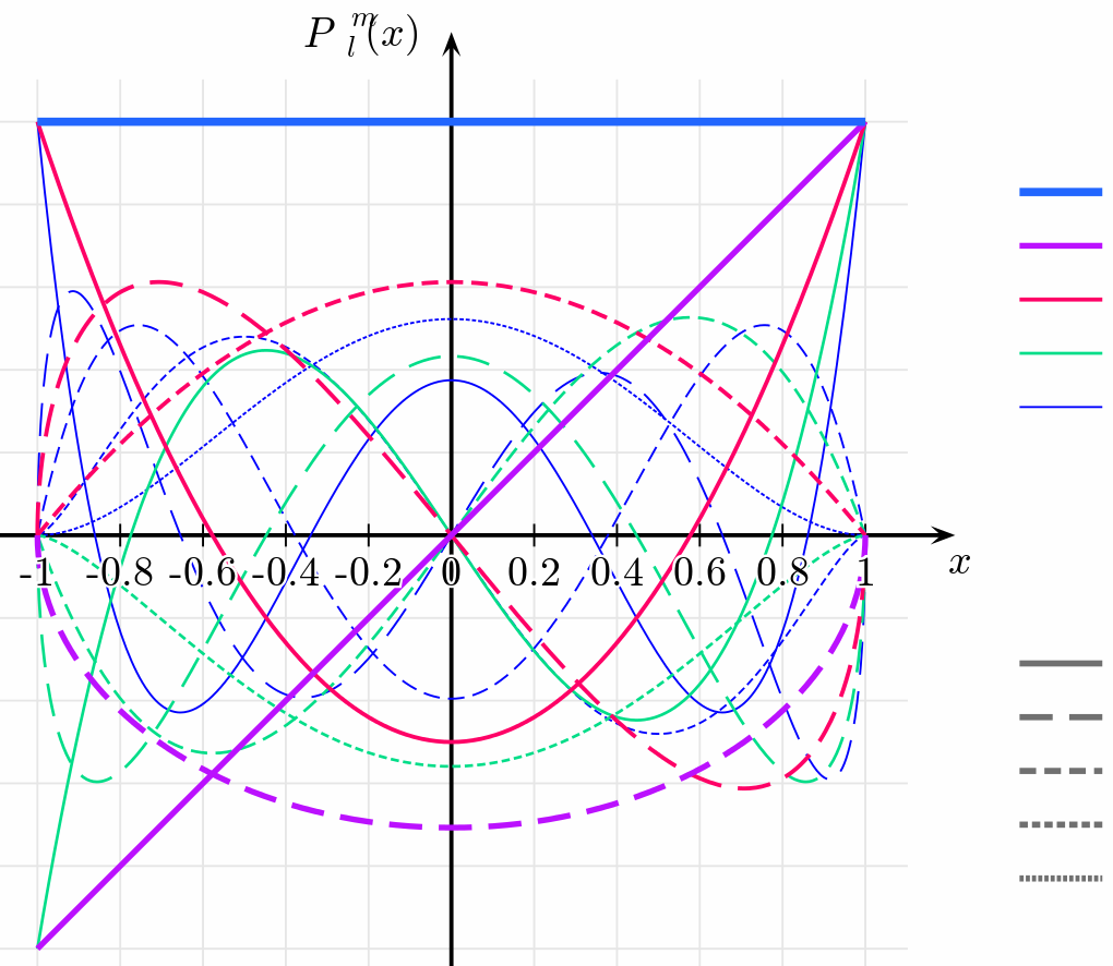
The reader should agree there is not much to fear in these functions – they are just certain sums of products of cos and sin (1 – 2)1/2. Fig. 25 shows the plots of a few lowest functions P nl ().
n
Pl
1
l 0
l 1
l 2
l 3
l 4
Fig. 2.25. A few lowest
associated Legendre functions.
(Adapted from an original by
n 0
Geek3,
available
at
n 1
https://en.wikipedia.org/wiki/Ass
n 2
ociated_Legendre_polynomials,
n 3
under
the
GNU
Free
n 4
Documentation License.)
1
Using the associated Legendre functions, the general solution (162) to the Laplace equation in the spherical coordinates may be expressed as
Variable
separation
l
in spherical
l
b
( r, ,) a r
l
n
.
(2.184) coordinates
P (cos) F ( ,)
F
( ) c cos n s sin n
l
l 1
l
n
(general
l0
r
n
n
n
n 0
case)
Since the difference between the angles and is somewhat artificial, physicists prefer to think not in terms of the functions P and F in separation, but directly about their products that participate in this solution.60
60 In quantum mechanics, it is more convenient to use a slightly different alternative set of basic functions of the same problem, namely the following complex functions called the spherical harmonics: 1/ 2
n
l
2
1 l
(
n)!
n
in
Y
( ,)
P (cos ) e
,
l
4
l
( n
l
)!
which are defined for both positive and negative n (within the limits – l n + l) – see, e.g., QM Secs. 3.6 and 5.6.
(Note again that in that field, our index n is traditionally denoted as m, and called the magnetic quantum number.) Chapter 2
Page 46 of 68


Essential Graduate Physics
EM: Classical Electrodynamics
As a rare exception for my courses, to save time I will skip giving an example of using the associated Legendre functions in electrostatics, because quite a few examples of these functions’
applications will be given in the quantum mechanics part of this series.
2.9. Charge images
So far, we have discussed various methods of solution of the Laplace boundary problem (35).
Let us now move on to the discussion of its generalization, the Poisson equation (1.41). We need it when besides conductors, we also have stand-alone charges with a known spatial distribution (r). (Its discussion will also allow us, better equipped, to revisit the Laplace problem in the next section.) Let us start with a somewhat limited, but very useful charge image (or “image charge”) method.
Consider a very simple problem: a single point charge near a conducting half-space – see Fig. 26.
z
q
r 1
r
'
r
d
0
r 2
0
Fig. 2.26. The simplest problem readily solvable by the
d
charge image method. The points’ colors are used, as
"
r
before, to denote the charges of the original (red) and
q
opposite (blue) sign.
Let us prove that its solution, above the conductor’s surface ( z 0), may be represented as: 1 q
q
q
1
1
r
( )
,
(2.185)
4
0 r
r
1
2
4 0 r ' r
r "
r
or in a more explicit form, using the cylindrical coordinates shown in Fig. 26:
q
1
1
(r)
,
(2.186)
4
1/ 2
1/ 2
2
0
( z 2
d)
2 ( z 2
d)
where is the distance of the field observation point r from the “vertical” line on which the charge is located. Indeed, this solution satisfies both the boundary condition = 0 at the surface of the conductor ( z = 0), and the Poisson equation (1.41), with the single -functional source at point r ’ = {0, 0, + d} on its right-hand side, because the second singularity of the solution, at point r ” = {0, 0, – d}, is outside the region of the solution’s validity ( z 0). Physically, this solution may be interpreted as the sum of the fields of the actual charge (+ q) at point r ’, and an equal but opposite charge (– q) at the “mirror image”
point r ” (Fig. 26). This is the basic idea of the charge image method.
Before moving on to more complex problems, let us discuss the situation shown in Fig. 26 in a little bit more detail, due to its fundamental importance. First, we can use Eqs. (3) and (186) to calculate the surface charge density:
Chapter 2
Page 47 of 68
EM: Classical Electrodynamics
q
1
1
q
2 d
. (2.187)
0
z 0
z
4 z
2
2
( z d) 1/2 2
2
( z d) 1/2
4
d
z0
2 23/2
From this, the total surface charge is
q
2 d
Q 2
d r 2 ()
d
d .
(2.188)
3 / 2
2
2
2
S
0
0
d
This integral may be easily worked out using the substitution 2/ d 2 (giving d = 2 d/ d 2): q
d
Q
q
(2.189)
2
3 / 2
0
.
1
This result is very natural: the conductor brings as much surface charge from its interior to the surface as necessary to fully compensate for the initial charge (+ q) and hence kill the electric field at large distances as efficiently as possible, hence reducing the total electrostatic energy (1.65) to the lowest possible value.
For a better feeling of this polarization charge of the surface, let us take our calculations to the extreme – to the q equal to one elementary change e, and place a particle with this charge (for example, a proton) at a macroscopic distance – say 1 m – from the conductor’s surface. Then, according to Eq.
(189), the total polarization charge of the surface equals that of an electron, and according to Eq. (187), its spatial extent is of the order of d 2 = 1 m2. This means that if we consider a much smaller part of the surface, A << d 2, its polarization charge magnitude Q = A is much less than one electron! For example, Eq. (187) shows that the polarization charge of quite a macroscopic area A = 1 cm2 right under the initial charge ( = 0) is e A/2 d 2 1.610-5 e. Can this be true, or our theory is somehow limited to the charges q much larger than e? (After all, the theory is substantially based on the approximate macroscopic model (1); maybe it is the culprit?)
Surprisingly enough, the answer to this question has become clear (at least to some physicists :-) only as late as in the mid-1980s when several experiments demonstrated, and theorists accepted (some of them rather grudgingly) that the usual polarization charge formulas are valid for elementary charges as well, i.e., such the polarization charge Q of a macroscopic surface area may differ from a multiple of e. The underlying reason for this paradox is the physical nature of the polarization charge of a conductor’s surface: as was discussed in Sec. 1, it is due not to new charged particles brought into the conductor (such charge would be in fact a multiple of e), but to a small shift of the free charges of a conductor by a very small distance from their equilibrium positions that they had in the absence of the external field induced by charge q. This shift is not quantized, at least on the scale relevant to our problem, and hence neither is Q.
This understanding has paved the way for the invention and experimental demonstration of several new devices including so-called single-electron transistors,61 which may be used, in particular, for ultrasensitive measurement of polarization charges as small as ~10-6 e. Another important class of single-electron devices is the dc and ac current standards based on the fundamental relation I = – ef, 61 Actually, this term (for which the author of these notes may be blamed :-) is misleading: the operation of the
“single-electron transistor” is based on the interplay of discrete charges (multiples of e) transferred between conductors, and sub-single-electron polarization charges – see, e.g., K. Likharev, Proc. IEEE 87, 606 (1999).
Chapter 2
Page 48 of 68
EM: Classical Electrodynamics
where I is the dc current carried by electrons transferred with the frequency f. The experimentally achieved62 relative accuracy of such standards is of the order of 10-7, and is not too far from that provided by the competing approach based on a combination of the Josephson effect and the quantum Hall effect.63
Second, let us find the potential energy U of the charge-to-surface interaction. For that, we may use the value of the electrostatic potential (185) at the point of the charge itself (r = r ’), of course ignoring the infinite potential created by the real charge, so the remaining potential is that of the image charge
1
q
( '
r )
.
(2.190)
image
4 2 d
0
Looking at the electrostatic potential’s definition given by Eq. (1.31), it may be tempting to immediately write U = qimage = – (1/40)( q 2/2 d) [WRONG!], but this would be incorrect. The reason is that the potential image is not independent of q, but is actually induced by this charge. This is why the correct approach is to calculate U from Eq. (1.61), with just one term:
1
1 q 2
U q
,
(2.191)
2
image
4 4 d
0
giving twice lower energy than the wrong result cited above. To double-check Eq. (191), and also get a better feeling of the factor ½ that distinguishes it from the wrong guess, we can calculate U as the integral of the force exerted on the charge by the conductor’s surface charge (i.e., in our formalism, by the image charge):
d
d
1
q 2
1 q 2
U F( z) dz
dz
.
(2.192)
4
(2 z)2
4 4 d
0
0
This calculation clearly accounts for the gradual build-up of the force F, as the real charge is being brought from afar (where we have opted for U =0) toward the surface.
This result has several important applications. For example, let us plot the electrostatic energy U
of an electron, i.e. a particle with charge q = – e, near a metallic surface, as a function of d. For that, we may use Eq. (191) until our macroscopic model (1) becomes invalid, and U transitions to some negative constant value (-) inside the conductor – see Fig. 27a. Since our calculation was for an electron with zero potential energy at infinity, at relatively low temperatures, k B T << , electrons in metals may occupy only the states with energies below – (the so-called Fermi level 64). The positive constant is called the workfunction because it describes the smallest work needed to remove the electron from a metal. As was discussed in Sec. 1, in good metals the electric field screening takes place at interatomic distances a 0 ~ 10-10 m. Plugging d = 110-10 m and q = – e –1.610-19 C into Eq. (191), we get
610–19 J 3.5 eV. This crude estimate is in surprisingly good agreement with the experimental values of the workfunction, ranging between 4 and 5 eV for most metals.65
62 See, e.g., M. Keller et al., Appl. Phys. Lett. 69, 1804 (1996) ; F. Stein et al., Metrologia 54, 1 (2017).
63 J. Brun-Pickard et al., Phys. Rev. X 6, 041051 (2016).
64 More discussion of these states may be found in SM Secs. 3.3 and 6.3.
65 More discussion of the workfunction, and its effect on the electrons’ kinetics, is given in SM Sec. 6.3.
Chapter 2
Page 49 of 68


Essential Graduate Physics
EM: Classical Electrodynamics
U
(a)
(b)
U
a 0
0
0
d
d
eE d
0
Fig. 2.27. (a) The origin
of the workfunction, and
1
(b) the field emission of
U
electrons (schematically).
d
Next, let us consider the effect of an additional uniform external electric field E0 applied normally to a metallic surface, on this potential profile. For that, we may the potential energy that the field gives to the electron at distance d from the surface, U ext = – eE 0 d, to that created by the image charge. (As we know from Eq. (1.53), since the field E0 is independent of the electron’s position, its recalculation into the potential energy does not require the coefficient ½.) As a result, the potential energy of an electron near the surface becomes
1
e 2
U ( d ) eE d
,
for d
0
>> a
4 4 d
0,
(2.193)
0
with a similar crossover to U = – inside the conductor – see Fig. 27b. One can see that at the appropriate sign, and a sufficient magnitude of the applied field, it lowers the potential barrier that prevents electrons from leaving the conductor. At E 0 ~ / a 0 (for metals, ~1010 V/m), this suppression becomes so strong that electrons with energies at, and just below the Fermi level start quantum-mechanical tunneling through the remaining thin barrier. This is the field electron emission (or just
“field emission”) effect, which is used in vacuum electronics to provide efficient cathodes that do not require heating to high temperatures.66
Returning to the basic electrostatics, let us find some other conductor geometries where the method of charge images may be effectively applied. First, let us consider a right-angle corner (Fig.
28a). Reflecting the initial charge in the vertical plane, we get the image shown in the top left corner of that panel. This image makes the boundary condition = const satisfied on the vertical surface of the corner. However, for the same to be true on the horizontal surface, we have to reflect both the initial charge and the image charge in the horizontal plane, flipping their signs. The final configuration of four charges, shown in Fig. 28a, satisfies all boundary conditions. The resulting potential distribution may be readily written as an evident generalization of Eq. (185). From it, the electric field and electric charge distributions, and the potential energy and forces acting on the charge may be calculated exactly as above – an easy exercise left for the reader.
Next, consider a corner with the angle /4 (Fig. 28b). Here we need to repeat the reflection operation not two but four times before we arrive at the final pattern of eight positive and negative charges. (Any attempt to continue this process would lead to overlap with the already existing charges.) 66 The practical use of such “cold” cathodes is affected by the fact that, as it follows from our discussion in Sec. 4, any nanoscale irregularity of a conducting surface (a protrusion, an atomic cluster, or even a single “adatom”
stuck to it) may cause a strong increase of the local field well above the applied uniform field E 0, making the electron emission reproducibility and stability in time significant challenges. In addition, the impact-ionization effects may lead to avalanche-type electric breakdown at dc fields as low as ~3106 V/m.
Chapter 2
Page 50 of 68


Essential Graduate Physics
EM: Classical Electrodynamics
This reasoning may be readily extended to corners of angles = / n, with any integer n, which require 2 n charges (including the initial one) to satisfy all the boundary conditions.
(a)
(b)
(c)
d
q
2 a d
q
q
q
q
q
x
q
q
q
q
q
0
a
2 a
(d)
(e)
Fig. 2.28. The charge images for (a, b) the corners with angles /2 and /4, (c) a plane capacitor, and (d) a rectangular box; (e) typical equipotential surfaces for the last system.
Some configurations require an infinite number of images but are still tractable. The most important of them is a system of two parallel conducting surfaces, i.e. an unbiased plane capacitor of infinite area (Fig. 28c). Here the repeated reflection leads to an infinite system of charges q at points x 2 aj d ,
(2.194)
j
where d (with 0 < d < a) is the position of the initial charge, and j is an arbitrary integer. The resulting infinite sum for the potential of the real charge q, created by the field of its images, 1
q
q
q 1
2
d
1
( d)
(2.195)
4 2 d
j
d x
d
a j j j d a
0
0
4
2
3
2
2
j
0
1
( / ,
)
is converging (in its last form) very fast. For example, the exact value, ( a/2) = –2ln2( q/40 a), differs by less than 5% from the approximation using just the first term of the sum.
Chapter 2
Page 51 of 68


Essential Graduate Physics
EM: Classical Electrodynamics
The same method may be applied to 2D (cylindrical) and 3D rectangular conducting boxes that require, respectively, 2D or 3D infinite rectangular lattices of images; for example in a 3D box with sides a, b, and c, charges q are located at points (Fig. 28d) r 2 ja 2 kb lc
2 '
r ,
(2.196)
jkl
where r ’ is the location of the initial (real) charge, and j, k, and l are arbitrary integers. Figure 28e shows a typical result of the summation of the potentials of this charge set, including the real one, in a 2D box (within the plane of the real charge). One can see that the equipotential surfaces, concentric near the charge, are naturally leaning along the conducting walls of the box, which have to be equipotential.
Even more surprisingly, the image charge method works very efficiently not only for rectilinear geometries but also for spherical ones. Indeed, let us consider a point charge q at distance d from the center of a conducting, grounded sphere of radius R (Fig. 29a), and try to satisfy the boundary condition
= 0 for the electrostatic potential on the sphere’s surface using an imaginary charge q’ located at some point beyond the surface, i.e. inside the sphere.
(a)
(b)
q, d
r