

Classical Electrodynamics by Konstantin K. Likharev - HTML preview
Download the book in PDF, ePub, Kindle for a complete version.
q' , d'
R
Fig. 2.29. Method of charge images for
0
a conducting sphere: (a) the idea, and
(b) the resulting potential distribution
in the central plane containing the
charge, for the particular case d = 2 R.
From the problem’s symmetry, it is clear that the point should be at the line passing through the real charge and the sphere’s center, at some distance d’ from the center. Then the total potential created by the two charges at an arbitrary point of free space, i.e. at r R (Fig. 29a) is
1
q
q'
( r, )
.
(2.197)
4
1/ 2
1/ 2
2
0
r 2
d 2 rd cos
2 r 2
d' 2 rd' cos
This expression shows that we can make the two involved fractions equal and opposite at all points on the sphere’s surface (i.e. for any at r = R) if we take67
R 2
R
d'
,
q' q .
(2.198)
d
d
Since the solution of any Poisson boundary problem is unique, Eqs. (197) and (198) give us the final solution for this problem. Fig. 29b shows a typical equipotential pattern following from this solution. It may be surprising how formulas that simple may describe such an elaborate field distribution.
67 In geometry, such points with dd’ = R 2, are referred to as the result of mutual inversion in a sphere of radius R.
Chapter 2
Page 52 of 68
EM: Classical Electrodynamics
Now we can calculate the total charge Q on the grounded sphere’s surface, induced by the external charge q. We could do this, as we have done for the conducting plane, by the brute-force integration of the surface charge density = –0/ r r = R. It is more elegant, however, to use the following Gauss law argument. Equality (197) is valid (at r R) regardless of whether we are dealing with our real problem (charge q and the conducting sphere) or with the equivalent charge configuration
– with the point charges q and q’, but no sphere at all. Hence, according to Eq. (1.16), the Gaussian integral over a surface with radius r = R + 0, and the total charge inside the sphere should be also the same. Hence we immediately get
R
Q q'
q .
(2.199)
d
A similar argumentation may be used to calculate the charge-to-sphere interaction force: 2
2
q'
q
R
1
q
Rd
F qE
( d) q
.
(2.200)
image
2
2
2
2
2 2
4 ( d d' )
4 d ( d R / d)
4 ( d R )
0
0
0
(Note that this expression is legitimate only at d > R.) At large distances, d >> R, this attractive force decreases as 1/ d 3. This unusual dependence arises because, as Eq. (199) specifies, the induced charge of the sphere, responsible for the force, is not constant but decreases as 1/ d. In the next chapter, we will see that such force is also typical for the interaction between a point charge and a dipole.
All previous formulas were for a sphere that is grounded to keep its potential equal to zero. But what if we keep the sphere galvanically insulated, so its net charge is fixed, for example, equals zero?
Instead of solving this problem from scratch, let us use (again!) the almighty linear superposition principle. For that, we may add to the previous problem an additional charge, equal to – Q = – q’, to the sphere, and argue that this addition gives, at all points, an additional, spherically symmetric potential that does not depend on the potential induced by the external charge q, and was calculated in Sec. 1.2 –
see Eq. (1.19). For the interaction force, such addition yields
2
qq'
qq'
q
Rd
R
F
.
(2.201)
2
2
2
2 2
3
4 ( d d')
4 πε d
4
( d
R )
d
0
0
0
At large distances, the two terms proportional to 1/ d 3 cancel each other, giving F 1/ d 5, so the potential energy of such interaction behaves as U 1/ d 4. Such a rapid force decay is due to the fact that the field of the uncharged sphere is equivalent to that of two (equal and opposite) induced charges + q’
and – q’, and the distance between them ( d – d’ = d – R 2/ d) tends to zero at d .
2.10. Green’s functions
I have spent so much time/space discussing potential distributions created by a single point charge in various conductor geometries because for any of the geometries, the generalization of these results to the arbitrary distribution (r) of free charges is straightforward. Namely, if a single charge q, located at some point r ’, creates at point r the electrostatic potential 1
(r)
qG(r, '
r ) ,
(2.202)
40
then, due to the linear superposition principle, an arbitrary charge distribution creates the potential Chapter 2
Page 53 of 68
EM: Classical Electrodynamics
1
1
Spatial
(r)
q G(r, r )
3
(r ) (r, r )
.
(2.203)
j
j
' G ' d r'
Green’s
4
4
0
j
0
function
The function G(r, r ’) is called the (spatial) Green’s function – the notion very fruitful and hence popular in all fields of physics.68 Evidently, as Eq. (1.35) shows, in the unlimited free space G r
( , '
r
1
)
,
(2.204)
r '
r
i.e. the Green’s function depends only on one scalar argument – the distance between the field-observation point r and the field-source (charge) point r ’. However, as soon as there are conductors around, the situation changes. In this course, I will only discuss Green’s functions defined to vanish as soon as the radius-vector r points to the surface ( S) of any conductor:69
G(r, '
r )
.
0
r S
(2.205)
With this definition, it is straightforward to deduce the Green’s functions for the solutions of the last section’s problems in which conductors were grounded, i.e. had potential = 0. For example, for a semi-space z 0 limited by a grounded conducting plane z = 0 (Fig. 26), Eq. (185) yields 1
1
G
,
with "
ρ '
ρ
and
z" z' ,
(2.206)
r '
r
r "
r
where is the 2D radius vector. We see that in the presence of conductors (and, as we will see later, any other polarizable media), Green’s function may depend not only on the difference r – r ’, but on each of these two arguments in a specific way.
So far, this is just re-naming our old results. The really non-trivial result of the Green’s function formalism in electrostatics is that, somewhat counter-intuitively, the knowledge of this function for a system with grounded conductors (Fig. 30a) enables the calculation of the field created by voltage-biased conductors (Fig. 30b), with the same geometry. To show this, let us use the so-called Green’s theorem of the vector calculus.70 The theorem states that for any two scalar, differentiable functions f(r) and g(r), and any volume V,
f 2 g
g 2 f d 3 r f g g f
d 2 r ,
(2.207)
n
V
S
where S is the surface limiting the volume. Applying the theorem to the electrostatic potential (r) and the Green’s function G (also considered as a function of r), let us use the Poisson equation (1.41) to replace 2 with (-/0), and notice that G, considered as a function of r, obeys the Poisson equation with the -functional source:
2
G(r, '
r ) 4 (r '
r ) .
(2.208)
68 See, e.g., CM Sec. 5.1, QM Secs. 2.2 and 7.4, and SM Sec. 5.5. Note that the numerical coefficient in Eq. (202) (and hence all resulting formulas) is the matter of convention; this choice does not affect the final results.
69 G so defined is sometimes called the Dirichlet function.
70 See, e.g., MA Eq. (12.3). Actually, this theorem is a ready corollary of the better-known divergence (“Gauss”) theorem, MA Eq. (12.2).
Chapter 2
Page 54 of 68


Essential Graduate Physics
EM: Classical Electrodynamics
(Indeed, according to its definition (202), this function may be formally considered as the field of a point charge q = 40.) Now swapping the notation of the radius-vectors, r r ’, and using the Green’s function symmetry, G(r, r ’) = G(r ’, r),71 we get
( ' r)
3
G(r, '
r )
( '
r )
4(r)
G(r, '
r ) d r'
2
( ' r)
G(r, '
r )
d r' .
(2.209)
n'
n'
V
0
S
(a)
(b)
0
1
0
q
q
2
2
2
q
q
q
j
q
j
1
1
Fig. 2.30. Green’s function method allows the solution of a simpler boundary problem (a) to be used for the solution of a more complex problem (b), for the same conductor geometry.
Let us apply this relation to the volume V of free space between the conductors, and the boundary S drawn immediately outside of their surfaces. In this case, by its definition, Green’s function G(r, r ’) vanishes at the conductor surface, i.e. at r S – see Eq. (205). Now changing the sign of ∂ n’ (so it would be the outer normal for conductors, rather than free space volume V), dividing all terms by 4, and partitioning the total surface S into the parts (numbered by index j) corresponding to different conductors (possibly, kept at different potentials k), we finally arrive at the famous result:72
1
Potential
3
1
G
(r, '
r )
(r)
( '
r G
) (r, '
r ) d r'
via Green’s
d 2 'r .
(2.210)
k
4
4
function
0
k
n'
V
Sk
While the first term on the right-hand side of this relation is a direct and evident expression of the superposition principle, given by Eq. (203), the second term is highly non-trivial: it describes the effect of conductors with arbitrary potentials k (Fig. 30b), using the Green’s function calculated for the similar system with grounded conductors, i.e. with all k = 0 (Fig. 30a). Let me emphasize that since our volume V excludes conductors, the first term on the right-hand side of Eq. (210) includes only the stand-alone charges in the system (in Fig. 30, marked q 1, q 2, etc.), but not the surface charges of the conductors
– which are taken into account, indirectly, by the second term.
In order to illustrate what a powerful tool Eq. (210) is, let us use to calculate the electrostatic field in two systems. In the first of them, a plane, circular, conducting disk of radius R, separated with a very thin cut from the remaining conducting plane, is biased with potential = V, while the rest of the plane is grounded – see Fig. 31.
71 This symmetry, evident for the particular cases (204) and (206), may be readily proved for the general case by applying Eq. (207) to the functions f (r) G(r, r ’) and g(r) G(r, r ” ). With this substitution, the left-hand side of that equality becomes equal to –4[ G(r ” , r ’) – G(r ’, r ” )], while the right-hand side is zero, due to Eq. (205).
72 In some textbooks, the sign before the surface integral is negative, because their authors use the outer normal to the free-space region V rather than those occupied by conductors – as I do.
Chapter 2
Page 55 of 68
EM: Classical Electrodynamics
z
'
r
r
0
V
0
0
R
"
r
Fig. 2.31. A voltage-biased conducting disk separated from the rest of a conducting plane.
If the width of the gap between the disk and the rest of the plane is negligible, we may apply Eq.
(210) without stand-alone charges, (r ’) = 0, and the Green’s function for the uncut plane – see Eq.
(206).73 In the cylindrical coordinates, with the origin at the disk’s center (Fig. 31), the function is 1
G(r, '
r )
2
2
2
'
2 '
cos( '
) ( z z' ) 1/2
1
.
(2.211)
2
2
2
'
2 '
cos( '
) ( z z' ) 1/2
(The sum of the first three terms under each square root in Eq. (211) is just the squared distance between the horizontal projections and ’ of the vectors r and r ’ (or r ” ) correspondingly, while the last terms are the squares of their vertical displacements.)
Now we can readily calculate the derivative participating in Eq. (210), for z 0: G
G
2 z
.
(2.212)
S
z' 0
n'
z'
2
2
2
'
2 '
cos( '
) z 3/2
Due to the axial symmetry of the system, we may take for zero. With this, Eqs. (210) and (212) yield V
2
R
G(r, r')
2
Vz
'd '
d r'
d '
.
(2.213)
4
n
2
'
2
' 2
2
'
cos '
z 2 3/2
S
0
0
This integral is not overly pleasing, but may be readily worked out at least for points on the symmetry axis ( = 0, z 0):74
2
R
R / 2
'd '
V
z
d
z
Vz
V
(2.214)
3 / 2
2
2
' z
R z
0
2
3 / 2
0
1
1
2 2 ,
1 / 2
This result shows that if z 0, the potential tends to V (as it should), while at z >> R, 2
R
V
.
(2.215)
2
2 z
73 Indeed, if all parts of the cut plane are grounded, a narrow cut does not change the field distribution, and hence the Green’s function, significantly.
74 There is no need to repeat the calculation for z 0: from the symmetry of the problem, (– z) = ( z).
Chapter 2
Page 56 of 68
EM: Classical Electrodynamics
Now let us use the same Eq. (210) to solve the (in :-)famous problem of the cut sphere (Fig. 32).
Again, if the gap between the two conducting semi-spheres is very thin ( t << R), we may use Green’s function for the grounded (and uncut) sphere. For a particular case r ’ = dn z, this function follows from Eqs. (197)-(198); generalizing the former relation for an arbitrary direction of vector r ’, we get 1
R / r'
G
,
for , , (2.216)
r 2 r' 2 2 rr' cos 1/2 r 2 ( R 2 / r' )2 2 r( R 2 / r' )cos
r r'
R
1/ 2
where is the angle between the vectors r and r ’, and hence r ” – see Fig. 32.
z
R
r
V
/ 2
'
r
"
r
t R
Fig. 2.32. A system of two separated, oppositely
biased semi-spheres.
V
/ 2
Now, calculating the Green’s function’s derivative,
2
2
G
( r R )
r'
,
(2.217)
R0
r'
R 2
2
r R 2 Rr cos 3/2
and plugging it into Eq. (210), we see that the integration is again easy only for the field on the symmetry axis (where r = zn z, and = ’), giving: 2
2
V
z R
1
.
(2.218)
2 z 2
2
z R
, for
0
1/ 2
For z R, this relation yields V/2 (as it should), while for z/ R , 3 R 2
V .
(2.219)
4 z 2
As will be discussed in the next chapter, such a field is typical for an electric dipole.
2.11. Numerical methods
Despite the richness of analytical methods, for many boundary problems (especially in geometries without a high degree of symmetry), the numerical approach is the only way to the solution.
Chapter 2
Page 57 of 68
EM: Classical Electrodynamics
Though software packages offering their automatic numerical solution are abundant nowadays,75 it is important for every educated physicist to understand “what is under the hood”, at least because most universal programs exhibit mediocre performance in comparison with custom codes written for particular problems, and sometimes do not converge at all, especially for fast-changing (say, exponential) functions. The very brief discussion presented here76 is a (hopefully, useful) fast glance under the hood, though it is certainly insufficient for professional numerical research work.
The simplest of the numerical approaches to the solution of partial differential equations, such as the Poisson or the Laplace equations (1.41)-(1.42), is the finite-difference method,77 in which the sought continuous scalar function f( r), such as the potential (r), is represented by its values in discrete points of a rectangular grid (frequently called mesh) of the corresponding dimensionality – see Fig. 33.
(a)
(b)
f
(c)
f
f
f
f
f
f
f
f
f
f
f
h
f
f
h
r
h
h
j
f
Fig. 2.33. The general idea of the finite-difference method in (a) one, (b) two, and (c) three dimensions.
Each partial second derivative of the function is approximated by the formula that readily follows from linear approximations of the function f and then its partial derivatives – see Fig. 33a: 2
f
f
1 f
f
1 f f
f f
f f 2 f
, (2.220)
2
r h / 2
r h / 2
2
r
r
r
h
r
j
r
j
h
h
h
h
j
j
j
j
j
where f f( rj + h) and f f( rj – h). (The relative error of this approximation is of the order of h 4∂4 f/∂ r 4 j.) As a result, the action of a 2D Laplace operator on the function f may be approximated as 2
2
f
f
f f 2 f
f f 2 f
f f f f 4 f
,
(2.221)
2
2
2
2
2
x
y
h
h
h
and of the 3D operator, as
2
2
2
f
f
f
f f f f f f 6 f
.
(2.222)
2
2
2
2
x
y
z
h
(The notation used in Eqs. (221)-(222) should be clear from Figs. 33b and 33c, respectively.) 75 See, for example, MA Secs. 16 (iii) and (iv).
76 It is almost similar to that given in CM Sec. 8.5 and is reproduced here for the reader’s convenience, illustrated with examples from this (EM) course.
77 For more details see, e.g., R. Leveque, Finite Difference Methods for Ordinary and Partial Differential Equations, SIAM, 2007.
Chapter 2
Page 58 of 68


Essential Graduate Physics
EM: Classical Electrodynamics
As a simple example, let us use this scheme to find the electrostatic potential distribution inside a cylindrical box with conducting walls and square cross-section a a, using an extremely coarse mesh with step h a / 2 (Fig. 34). In this case, our function, the electrostatic potential ( x, y), equals zero at the side and bottom walls, and V 0 at the top lid, so, according to Eq. (221), the 2D Laplace equation may be approximated as
0 0 V 0 4
0
.
0
(2.223)
( a / )
2 2
The resulting value for the potential in the center of the box is = V 0/4.
V
0
a / 2
a
Fig. 2.34. Numerically solving an internal 2D boundary
2
problem for a conducting, cylindrical box with a square
cross-section, using a very coarse mesh (with h = a/2).
0
Surprisingly, this is the exact value! This may be proved either by solving this problem by the variable separation method, just as this has been done for a similar 3D problem in Sec. 5, or just from the following Green’s-function argument. If all four walls of our 2D volume were biased to the voltage V 0, there would be no electric field in it at all, so the middle-point potential would be equal to V 0 as well.
However, from the point of view of Eq. (210) with no bulk charge, (r) = 0, this result may be legitimately viewed as the linear superposition of the four contributions of the potentials k = V 0 of each wall. Since for this symmetric geometry, the corresponding geometrical factors are equal, the contribution of one wall, with k = 0 on all other walls (as in our current problem), has to equal V 0/4.
For a similar 3D problem (a cubic box), with a similar 3D mesh, Eq. (222) yields
0 0 V 0 0 0 6
0
0,
(2.226)
( a / 2)2
so = V 0/6. Using the same Green’s-function argument, now for six walls of the cube, we see that this result is also exact! (This fact also follows from our variable-separation result expressed by Eqs. (95) and (99) with a = b = c.)
Though such exact results should be considered as a happy coincidence rather than the general law, they still show that numerical methods, even with relatively crude meshes, may be more computationally efficient than some “analytical” approaches, like the variable separation method with its infinite-sum results that, in most cases, require computers anyway – at least for the result’s comprehension and analysis.
A more powerful (but also much more complex) approach is the finite-element method in which the discrete point mesh, typically with triangular cells, is (automatically) generated in accordance with the system geometry.78 Such mesh generators provide higher point concentration near sharp convex 78 See, e.g., CM Fig. 8.14.
Chapter 2
Page 59 of 68


Essential Graduate Physics
EM: Classical Electrodynamics
parts of conductor surfaces, where the field concentrates and hence the potential changes faster, thus ensuring a better accuracy-to-speed tradeoff than the finite-difference methods on a uniform grid. The price to pay for this improvement is the algorithm’s complexity which makes its adjustments much harder. Unfortunately, in this series, I do not have time for going into the details of that method and have to refer the reader to the special literature on this subject.79
2.12. Exercise problems
2.1. Calculate the force (per unit area) exerted on a conducting surface by an external electric field normal to it. Compare the result with the electric field’s definition given by Eq. (1.6), and comment.
QB
S
4
S 3
Q
2.2. Electric charges Q
A
A and QB have been placed on two conducting
S 2
concentric spherical shells – see the figure on the right. What is the full S 1
charge of each of the surfaces S 1- S 4?
C
C
1
2
2.3. Calculate the mutual capacitance between the terminals of the
lumped-capacitor circuit shown in the figure on the right. Analyze and
C
interpret the result for major particular cases.
0
C
C
2
1
C
C
C
1
1
1
2.4. Calculate the mutual capacitance between the terminals
of the semi-infinite lumped-capacitor circuit shown in the figure on
the right, and find the law of the applied voltage’s decay along the
C
C
C
2
2
2
system. Analyze and interpret the result.
A 1
2.5. A system of two thin conducting plates is located over a
A
ground plane as shown in the figure on the right, where A
2
1 and A 2 are
the areas of the indicated plate parts, while d’ and d” are the distances 1
between them. Neglecting the fringe effects, calculate:
d'
2
(i) the effective capacitance of each plate, and
d"
(ii) their mutual capacitance.
79 See, e.g., either C. Johnson, Numerical Solution of Partial Differential Equations by the Finite Element Method, Dover, 2009, or T. Hughes, The Finite Element Method, Dover, 2000.
Chapter 2
Page 60 of 68




Essential Graduate Physics
EM: Classical Electrodynamics
2.6. A wide and thin film carrying a uniformly distributed
electric charge of areal density is placed inside a plane capacitor
whose plates are connected with a wire – see the figure on the right.
t
Neglecting the fringe effects, calculate the surface charges of the plates
d
and the net force exerted on the film (per unit area).
2.7. A relatively small conductor (possibly, of an
irregular shape) with self-capacitance C is located at distance
r from the center of a conducting sphere of radius R – see the
R
r
C
figure on the right. In the first approximation in C, find the
reciprocal capacitance matrix of the system. Use the matrix to
calculate its potential energy and the force of the conductor
interaction for two cases:
(i) the conductor charges Q are equal, and
(ii) the conductor potentials are kept equal.
2.8. Use the Gauss law to calculate the mutual capacitance of the
following two-electrode systems, both with the cross-section shown in Fig. 7
b a
(reproduced on the right):
(i) a conducting sphere in the center of a spherical cavity inside
another conductor, and
0
a
(ii) a long conducting round cylinder on the axis of a cylindrical cavity
inside another conductor, i.e. a coaxial cable. (In this case, we speak about the
capacitance per unit length).
Compare the results with those obtained in Sec. 2.2 using the Laplace
equation.
2.9. Calculate the electrostatic potential distribution around two barely
V
0
separated conductors in the form of coaxial round cones (see the figure on the 2
right), with voltage V between them. Compare the result with that of a similar 2D
problem, with the cones replaced with plane-face wedges. Can you calculate the
V
mutual capacitances between the conductors in these systems? If not, can you 2
estimate them?
2.10. Calculate the mutual capacitance between two
rectangular planar electrodes of area A = a l, with a very small 0
angle 0 between them – see the figure on the right.
0
a
0
0
2.11. Using the results for a single thin round disk, obtained in Sec. 4,
R
consider a system of two such disks at a small distance d << R from each other d
– see the figure on the right. In particular, calculate:
(i) the reciprocal capacitance matrix of the system,
Chapter 2
Page 61 of 68


Essential Graduate Physics
EM: Classical Electrodynamics
(ii) the mutual capacitance between the disks,
(iii) the partial capacitance of one disk, and
(iv) the effective capacitance of one disk,
– all in the first nonvanishing approximation in d/ R << 1. Compare the results (ii)-(iv) and interpret their similarities and differences.
2.12.* Calculate the mutual capacitance (per unit length) between
two cylindrical conductors forming a system with the cross-section shown
R
in the figure on the right, in the limit t << w << R.
Hint: You may like to use the elliptic coordinates mentioned in Sec.
t
4. They are defined by the following equality:
w
x iy c cosh( i ),
(*)
where c is a constant.
2.13. Calculate the mutual capacitance (per unit length) between two similar, long, parallel wires, each with a round cross-section of radius R, whose axes are separated by distance d > 2 R. Explore and interpret the result in the limits R 0 and R 2 d.
Hint: You may like to use the 2D orthogonal bipolar coordinates {, } defined by the following relations with the Cartesian coordinates { x, y}:
sinh
sin
x a
,
y a
,
with ,
.
cosh cos
cosh cos
In these coordinates, the Laplace operator is
2
2
2 1 cosh cos
.
2
2
2
a
2.14. Formulate 2D electrostatic problems that may be simply solved using each of the following analytic functions of the complex variable z x + iy:
(i) w = ln z,
(ii) w = z1/2,
(iii) w = z + 1/z,
and solve these problems.
2.15. On each side of a cylindrical volume with a rectangular cross-section a b, with no electric charges inside it, the electric field’s component normal to the side’s plane is constant, and also equal and opposite to that on the opposite side. Calculate the distribution of the electric potential inside the volume, provided that the magnitude of the normal components on the sides of length b equals E.
Suggest a practicable method to implement such potential distribution.
2.16. Complete the solution of the problem shown in Fig. 12, by calculating the distribution of the surface charge on the semi-planes. Can you calculate the mutual capacitance between the semi-planes (per unit length of the system)? If not, can you estimate it?
Chapter 2
Page 62 of 68


Essential Graduate Physics
EM: Classical Electrodynamics
2.17. A straight, long, thin, round-cylindrical conducting pipe has been
V / 2
cut, along its axis, into two equal parts – see the figure on the right.
(i) Use the conformal mapping method to calculate the distributions of
R
the electrostatic potential created by voltage V applied between the two parts, both outside and inside the pipe, and of the surface charge.
(ii)* Calculate the mutual capacitance between the pipe’s halves (per
unit length), taking into account a small width 2 t << R of the cut.
Hints: In Task (i), you may like to use the complex function
R z
V / 2
w ln
,
R z
while in Task (ii), you may use the solution of the previous problem.
0
2.18. A gap of constant width w between two grounded conducting semi-spaces is closed, from one side, with a conducting plunger biased with voltage V, so that the w
cross-section of the system looks like the figure on the right shows. Use the variable separation method to calculate the distribution of the electrostatic potential within the gap.
V
V / 2
2.19. Use the variable separation method to calculate the electrostatic
a
a
potential’s distribution inside a very long thin-wall metallic box with a quadratic cross-section, cut and voltage-biased as shown in the figure on the right. (Assume a
a
that the cut’s width is negligibly small.)
V / 2
2.20. Solve Problem 17(i) by using the variable separation method, and compare the results.
2.21. Use the variable separation method to calculate the potential distribution above the plane surface of a conductor, with a strip of width w separated by very thin cuts, and biased with voltage V –
see the figure below.
w
V
0
0
2.22. The previous problem is now modified: the cut-out and voltage-biased part of the conducting plane is now not a strip, but a square with side w. Calculate the potential distribution above the conductor’s surface.
Chapter 2
Page 63 of 68
EM: Classical Electrodynamics
V
V
V
2.23. Each electrode of a large plane capacitor is cut into
2
2
2
parallel long strips of equal width w, with very narrow gaps
between them. These strips are kept at alternating potentials, as
w
d
shown in the figure on the right. Use the variable separation
method to calculate the electrostatic potential distribution in space,
V
V
V
and explore the limit w << d.
2
2
2
2.24. Complete the cylinder problem started in Sec. 7 (see Fig. 17), for the cases when the top lid’s voltage is fixed as follows:
(i) V = V 0 J 1(11/ R) sin, where 11 3.832 is the first root of the Bessel function J 1(); (ii) V = V 0 = const.
For both cases, calculate the electric field at the centers of the lower and upper lids. (For Task (ii), an answer including series and/or integrals is acceptable.)
2.25. For the infinitely long periodic system sketched in Fig. 21, assuming that t << h, R: (i) calculate and sketch the electrostatic potential’s distribution inside the system for various values of the ratio R/ h, and
(ii) simplify the results for the limit R/ h 0.
2.26. A long round cylindrical conducting pipe is split, with a
V / 2
V / 2
very narrow cut normal to its axis, into two parts that are voltage-
biased as the figure on the right shows. Use two different approaches 2 R
to calculate the force exerted by the resulting field upon a charged
particle flying along the pipe close to its axis. Can the system work as
an electrostatic lens?
2.27. Use the variable separation method to find the potential distribution inside and outside of a thin spherical shell of radius R, with a fixed potential distribution on it: ( R,,) = V 0 sin cos.
2.28. A thin spherical shell carries an electric charge with areal density = 0cos. Calculate the spatial distribution of the electrostatic potential and the electric field, both inside and outside the shell.
2.29. Use the variable separation method to solve the problem already considered in Sec. 10: calculate the potential distribution both inside and outside of a thin spherical shell of radius R, separated with a very thin cut along the central plane z = 0 into two halves, with voltage V applied between them –
see Fig. 32. Analyze the solution; in particular, compare the field at the z-axis, for z > R, with Eq. (218).
Hint: You may like to use the following integral of a Legendre polynomial with an odd index l =
1, 3, 5…= 2 n – 1:80
80 As a reminder, the double factorial (also called “semifactorial”) operator (!!) is similar to the usual factorial operator (!), but with the product limited to numbers of the same parity as its argument – in our particular case, of the odd numbers in the numerator and even numbers in the denominator.
Chapter 2
Page 64 of 68


Essential Graduate Physics
EM: Classical Electrodynamics
1
n
n
I P
d
.
n
n
n
2
1
1
1
3
5
3
...
1 2
3 !
!
1
n! 2 2 2
2
2 n 2 n 2 !
!
0
z
V
d
2.30. Calculate, up to terms O(1/ r 2), the long-range electric field induced by a split and voltage-biased conducting sphere – similar to that discussed in Sec. 10
R
0
(see Fig. 32) and in the previous problem, but with the cut’s plane at an arbitrary distance d < R from the center – see the figure on the right.
0
2.31. Calculate the field distribution in the simple electrostatic lens that was the subject of Problem 1.9, provided that the separation of the two field regions is provided by a thin conducting membrane, with a round hole of radius R.
Hint: You may like to use the fact that the general axially symmetric solution of the Laplace equation in the oblate ellipsoidal coordinates (59) may be represented in the following variable-separation form:
p P i
q Q i
,
n
n sinh
n
n sinh P n cos
n0
where pn and qn are constants, Pn are the Legendre polynomials (2.169), which are sometimes called the Legendre functions of the first kind, while Qn are the Legendre functions of the second kind (briefly mentioned, in a different context, in Sec. 2.8) that may be defined by the following recurrence relations:
Q
Q P Q
Q
n
Q n
Q
0
1 1
ln
,
1
1 0
,
1
n2
2
1
n 1
1
n2 .
2 1
n
n
2.32. A small conductor (in this context, usually called a single-
V
electron island) is placed between two conducting electrodes, with
voltage V applied between them. The gap between the island and one of
the electrodes is so narrow that electrons may tunnel quantum-
"island"
mechanically through this “junction” – see the figure on the right.
tunnel
Neglecting thermal excitation effects, calculate the equilibrium charge of
junction
the island as a function of V.
Hint: To solve this problem, you do not need to know much about
0
the quantum-mechanical tunneling between conductors, besides that such tunneling of an electron, together with energy relaxation of the resulting excitations, may be considered a single inelastic (energy-dissipating) event.81 At negligible thermal excitations, such an event takes place only if it decreases the total potential energy of the system.
81 Strictly speaking, this statement, implying negligible quantum-mechanical coherence of the tunneling events, is correct only if the junction transparency is so low that its effective electric resistance is much higher than the fundamental quantum unit of resistance, R Q /2 e 2 6.5 k (see, e.g., QM Sec. 3.2). However, this condition is satisfied in most experimental tunnel junctions.
Chapter 2
Page 65 of 68





Essential Graduate Physics
EM: Classical Electrodynamics
V
2.33. The system discussed in the previous problem is now
generalized as the figure on the right shows. If the voltage V’ applied between the two bottom electrodes is sufficiently large, electrons can successively tunnel through two junctions of this system (called the single-electron
"
island"
transistor), carrying dc current between these electrodes. Neglecting thermal excitations, calculate the region of voltages V and V’ where such a current is fully suppressed ( Coulomb-blocked).
V' tunnel 0
junctions
2.34. Use the charge image method to calculate the full surface charges induced in the plates of a very broad, voltage-unbiased plane capacitor of thickness D by a point charge q separated from one of the electrodes by distance d. Suggest at least one alternative method to obtain the same result.
2.35. Use the charge image method to calculate the potential energy of the electrostatic interaction between a point charge placed in the center of a spherical cavity that had been carved inside a grounded conductor, and the cavity’s walls. Looking at the result, could it be obtained in a simpler way (or ways)?
2.36. Use the method of charge images to find the Green’s
R
function of the system shown in the figure on the right, where the
bulge on the (otherwise, plane) surface of a conductor has the shape
of a semi-sphere of radius R.
2.37.* Use the spherical inversion expressed by Eq. (198), to develop an iterative method for a more and more precise calculation of the mutual capacitance between two similar conducting spheres of radius R, with their centers separated by distance d > 2 R.
R 1
2.38.* A conducting sphere of radius R 1, carrying an electric charge Q, is R
placed inside a spherical cavity of radius R
2
2 > R 1, carved inside another bulk
conductor. Calculate the electric force exerted on the sphere if its center is
Q
displaced by a small distance << R 1, R 2 – R 1 from that of the cavity – see the figure on the right.
2.39. Within the simple models of the electric field screening in conductors, discussed in Sec.
2.1, analyze the partial screening of the electric field of a point charge q by a planar conducting film of constant thickness t << , where is (depending on charge carrier statistics) either the Debye or the Thomas-Fermi screening length – see, respectively, Eqs. (8) or (10). Assume that the distance d between the charge and the film is much larger than t.
2.40. Prove the following expansion of the simplest Green’s function (204) into a series over the Legendre polynomials:
Chapter 2
Page 66 of 68
EM: Classical Electrodynamics
l
1
1
r
P (cos ,)
r
l
'
r
r
r
l0
where r> is the largest of the two scalars r r 0 and r’ r ’ 0, while r< is the smallest of them.
2.41. Use the expansion that was the subject of the previous problem to confirm the analysis, in Sec. 2.9 of the lecture notes, of the system shown in Fig. 29: a grounded conducting sphere of radius R, and a point charge q located at distance d > R from its center.
2.42. Suggest a convenient definition of the Green’s function for 2D electrostatic problems, and calculate it for:
(i) the unlimited free space, and
(ii) the free space above a conducting plane.
Use the latter result to re-solve Problem 21.
2.43. A conducting plane is separated into two parts with a very narrow straight cut, and voltage V is applied between the resulting half-planes – see the figure below. Use the Green’s function method to find the distribution of the electrostatic potential and the electric field everywhere in the space.
Compare the result with Eq. (83). In hindsight, could the problem be solved in an even simpler way (or ways)?
V
/ 2
V
/ 2
2.44. Use the last result of Problem 42 and one of the conformal mappings discussed in Sec. 4 to find one more solution of Problem 18.
2.45. Calculate the 2D Green’s functions for the free spaces:
(i) outside a round conducting cylinder, and
(ii) inside a round cylindrical hole in a conductor.
2.46. Solve Problem 17(i) using the Green’s function method.
2.47. Solve the 2D boundary problem that was discussed in Sec. 11 (Fig. 34) by using: (i) the finite difference method with the finer square mesh h = a/3, and (ii) the variable separation method.
Compare the results at the mesh points, and comment.
Chapter 2
Page 67 of 68
EM: Classical Electrodynamics
This page is
intentionally left
blank
Chapter 2
Page 68 of 68


Essential Graduate Physics
EM: Classical Electrodynamics
Chapter 3. Dipoles and Dielectrics
In contrast to conductors, the motion of charges in dielectrics is restricted to the atom/molecule interiors, so the electric polarization of these materials by an external field takes a different form. This issue is the main subject of this chapter, but in preparation for its analysis, we have to start with a general discussion of the electric field induced by spatially restricted systems of charges.
3.1. Electric dipole
Let us consider a localized system of charges, of a linear scale a, and derive a simple approximate expression for the electrostatic field induced by the system at a distant point r. For that, let us select a reference frame with the origin either somewhere inside the system, or at a distance of the order of a from it (Fig. 1).
r
'
r
a
0
Fig. 3.1. Deriving the approximate expression
for the electrostatic field of a localized system
of charges at a distant point ( r >> r’ ~ a).
Then the positions of all charges of the system satisfy the following condition:
r' r .
(3.1)
Using this condition, we can expand the general expression (1.38) for the electrostatic potential (r) of the system into the Taylor series in small parameter r’. For any function of type f (r – r ’), the expansion may be represented as1
3
f
1 3
2
f
f (r '
r ) f (r) r '
(r)
r 'r '
r
.
(3.2)
j
'
r
( )
...
0
j
j'
'
r
j
r
r r
j
j j'
1
!
2
0
,
1
j
j'
Applying this formula to the fraction 1/r – r ’ in Eq. (1.38) (i.e. essentially to the free-space Green’s function), we get the so-called multipole expansion of the electrostatic potential: 1 1
1 3
1
3
r
Q
r p
r r Q
,
(3.3)
3
j
j
5
...
j j'
jj'
4
r
r
r
0
j1
2
j,j' 1
whose r-independent parameters are defined as follows:
Q '
r d 3 r' ,
p
3
2
3
r
,
Q
r 3
.
(3.4)
j
' r 'd r'
j
jj'
'
r 'r ' r'
j
j'
jj' d r'
1 See, e.g., MA Eq. (2.11b).
© K. Likharev
Essential Graduate Physics
EM: Classical Electrodynamics
(Indeed, the two leading terms of the expansion (2) may be rewritten in the vector form f(r) – r ’ f(r), and the gradient of such a spherically-symmetric function f( r) = 1/ r is just n rdf/ dr, so 1
1
d 1 1
r
'
r n
'
r
,
(3.5)
r
3
r '
r
r
dr r r
r
immediately giving the two first terms of Eq. (3). The proof of the third, quadrupole term in Eq. (3) is similar but a bit longer, and is left for the reader’s exercise.)
Evidently, the scalar parameter Q in Eqs. (3)-(4) is just the total charge of the system. The constants pj may be considered as Cartesian components of the following vector: Electric
p ( ' r 'd 3
)r
r' ,
(3.6)
dipole
moment
called the system’s electric dipole moment, and Q jj’ are Cartesian elements of a tensor – system’s electric quadrupole moment. If Q 0, all higher terms on the right-hand side of Eq. (3), at large distances (1), are just small corrections to the first one, and in many cases may be ignored. However, the net charge of many systems is exactly zero, the most important examples being neutral atoms and molecules. For such neural systems, the second ( dipole) term in Eq. (3) is, most frequently, the leading one. Such systems are called electric dipoles. Due to their importance, let us rewrite the expression for the dipole term in three other, mathematically equivalent forms:
1 r p
1
p cos
1
pz
Electric
,
(3.7)
dipole’s
d
3
2
4
r
4
r
4
potential
0
0
0 2
2
2
x y z 3/2
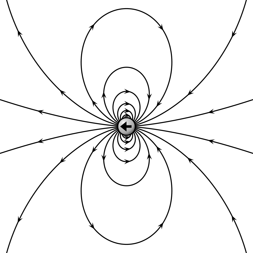
that are more convenient for some applications. Here is the angle between the vectors p and r, and in the last (Cartesian) representation, the z-axis is directed along the vector p. Fig. 2a shows equipotential surfaces of the dipole field – or rather their cross-sections by any plane in which the vector p resides.
p
(a)
(b)
p
r
r
E r
Fig. 3.2. (a) The equipotential surfaces and (b) the electric field lines of a dipole. (Panel (b) adapted from http://en.wikipedia.org/wiki/Dipole under the GNU Free Documentation License.) Chapter 3
Page 2 of 28
EM: Classical Electrodynamics
The simplest example of a system whose field, at large distances, approaches the dipole field (7), is two equal but opposite point charges (“poles”), + q and – q, with the radius vectors, respectively, r+
and r–:
r ( q) (r r ) ( q) (r r ) .
(3.8)
For this system (sometimes called the physical dipole), Eq. (4) yields
p ( q r
) ( q r
)
q r
( r ) qa ,
(3.9)
where a is the vector connecting the points r- and r+. Note that in this case (and indeed for all systems with Q = 0), the dipole moment does not depend on the choice of the reference frame’s origin.
A less trivial example of a dipole is a conducting sphere of radius R in a uniform external electric field E0. As a reminder, its field was calculated in Sec. 2.8, and its result is expressed by Eq. (2.176).
The first term in the parentheses of that relation describes just the external field (2.173), so the field of the sphere itself (i.e. that of the surface charge induced by E0) is given by the second term: 3
E R
0
cos .
(3.10)
s
2
r
Comparing this expression with the second form of Eq. (7), we see that the sphere has an induced dipole moment
p 4
3
E R .
(3.11)
0
0
This is an interesting example of a virtually pure dipole field: at all points outside the sphere ( r > R), the field has neither a quadrupole moment nor any higher moments.
Other examples of dipole fields are given by two more systems discussed in Chapter 2 – see Eqs.
(2.215) and (2.219). Those systems, however, do have higher-order multipole moments, so for them, Eq.
(7) gives only the long-distance approximation.
Now returning to the general properties of the dipole field (7), let us calculate its major characteristics. First of all, we may use Eq. (7) to calculate the electric field of a dipole: 1
r p
1
p cos
E
.
(3.12)
d
d
4
3
r
4
r
0
2
0
This differentiation is easiest in the spherical coordinates, using the well-known expression for the gradient of a scalar function in these coordinates2 and taking the z-axis parallel to the dipole moment p.
From the last form of Eq. (12), we immediately get
Electric
2
p
1 3r(r p) p r
dipole’s
E
2n cos n sin
.
(3.13)
d
r
3
5
field
4 r
4
r
0
0
Fig. 2b above shows the electric field lines given by Eqs. (13). The most important features of this result are a faster drop of the field’s magnitude ( E d 1/ r 3, rather than E 1/ r 2 for a point charge), and the change of the signs of its radial component as a function of the polar angle [0, ].
2 See, e.g., MA Eq. (10.8) with / = 0.
Chapter 3
Page 3 of 28
EM: Classical Electrodynamics
Next, let us use Eq. (1.55) to calculate the potential energy of interaction between a dipole and an external electric field. Assuming that this field does not change much at distances of the order of a (Fig. 1), we may expand its potential ext(r) into the Taylor series, and keep only two leading terms: 3
U (r) (r) d r (r) (0) r (0) d r Q
0 p E
.
(3.14)
ext
ext
3
ext
ext
ext
The first term is the potential energy the system would have if it were just a point charge. If the net charge Q is zero, that term disappears, and the leading contribution is due to the dipole moment: U p E ,
for p const .
(3.15a)
ext
Note that this result is only valid for a fixed dipole, with p independent of E
Dipole’s
ext. In the opposite limit, energy in
when the dipole is induced by the field, i.e. p Eext (you may have one more look at Eq. (11) to see an external example of such a proportionality), we need to start with Eq. (1.60) rather than Eq. (1.55), getting field
1
U p E ,
for p
E .
(3.15b)
ext
ext
2
In particular, combining Eqs. (13) and Eq. (15a), we may get the following important formula for the interaction of two independent dipoles:
2
1 p p r (
3 r p )(r p )
1
p p p p 2 p p
1 x
2 x
1 y
2 y
1 z
2
1
2
1
2
U
z
,
(3.16)
int
5
3
4
r
4
r
0
0
where r is the vector connecting the dipoles, and the z-axis is directed along this vector. It is easy to prove (this exercise is left for the reader) that if the magnitude p of each dipole moment is fixed (the approximation valid, in particular, for weak interaction of so-called polar molecules), this potential energy reaches its minimum at the parallel orientation of the dipoles along the line connecting them.
Note also that in this case, U int is proportional to 1/ r 3. On the other hand, if each moment p has a random value plus a component due to its polarization by the electric field of its counterpart: p1,2 E2,1 1/ r 3, their average interaction energy (which may be calculated from Eq. (16) with the additional factor ½) is always negative and is proportional to 1/ r 6. Such negative potential describes, in particular, the long-range, attractive part (the so-called London dispersion force) of the interaction between electrically neutral atoms and molecules.3
According to Eqs. (15), the electric field should “try” to reach the minimum of U by aligning the dipole vector’s direction with its own. The direct quantitative description of this effect is the torque
exerted by the field. The simplest way to calculate it is to sum up all the elementary torques d = r dFext
= rEext(r)(r) d 3 r exerted on all elementary charges of the system: τ r E (r)(r) 3
d r p E ( )
0 ,
(3.17)
ext
ext
where at the last step, the spatial dependence of the external field Eext(r) was again neglected. This dependence cannot, however, be ignored at the calculation of the total force exerted by the field on the dipole (with Q = 0). Indeed, Eqs. (15) shows that if the field is constant, the dipole’s energy is 3 Several calculations of this force, using various models, are described in the QM and SM parts of this series.
Chapter 3
Page 4 of 28
EM: Classical Electrodynamics
independent of its spatial location and hence the net force is zero. However, if the field has a non-zero gradient, a total force does appear; for a field-independent dipole,
F U (p E ) ,
(3.18)
ext
where the derivative has to be taken at the dipole’s position (in our notation, at r = 0). If the dipole that is being moved in a field retains its magnitude and orientation, then the last formula is equivalent to4
F p E .
(3.19)
ext
Alternatively, the last expression may be obtained similarly to Eq. (14):
F
3
(r)E (r) d r (r) E 0 (r )E
d r
QE (0) (p )E
.
(3.20)
ext
ext
ext
3
ext
ext
Finally, let me add a note on the so-called coarse-grain model of the dipole. The dipole approximation explored above is asymptotically correct only at large distances, r >> a. However, for some applications (including the forthcoming discussion of the molecular field effects in Sec. 3) it is beneficial to have an expression that might be formally used everywhere in space, though maybe without exact details at r ~ a, giving the correct result for the space average of the electric field, 1
E
E d 3 r ,
(3.21)
V V
where V is a regularly-shaped volume much larger than a 3, for example, a sphere of radius R >> a, with the dipole at its center. For the field Ed given by Eq. (13), such an average is zero. Indeed, let us consider the Cartesian components of that vector in a reference frame with the z-axis directed along the vector p. Due to the axial symmetry of the field, the averages of the components Ex and Ey vanish. Let us use Eq. (13) to spell out the “vertical” component of the field (parallel to the dipole moment vector): p
1
p
E E
2n p cos n p sin
2cos
sin
.
(3.22)
z
d
r
2
2
p
3
4
r
3
4
r
0
0
Integrating this expression over the whole solid angle = 4, at fixed r, using a convenient variable substitution cos , we get
1
p
p
E d Ω 2 E sin d
. (3.23)
z
z
2cos2 sin2sin d
3 2
1 d 0
2
3
r
2
3
r
4
0
0
0
0
1
On the other hand, the exact electric field of an arbitrary charge distribution, with the total dipole moment p, obeys the following equality:
3
p
1 4
E r
( ) d r
p
,
(3.24)
3
4
3
V
0
0
where the integration is over any sphere containing all the charges. (A proof of this formula by using Eqs. (1.9) and (1.22) is left for the reader’s exercise.) The origin of the difference is illustrated in Fig. 3
on the example of a physical dipole, i.e. a system of two equal but opposite charges – see Eqs. (8)-(9).
4 The equivalence may be proved, for example, by using MA Eq. (11.6) with f = p = const and g = Eext, taking into account that according to the general Eq. (1.28), Eext = 0.
Chapter 3
Page 5 of 28


Essential Graduate Physics
EM: Classical Electrodynamics
The zero average (23) of the dipole field (13) does not take into account the contribution from the region between the charges where Eq. (13) is not valid, and the field is directed mostly against the dipole vector (9).
p
E
V
q
q
Fig. 3.3. A sketch illustrating the origin
of Eq. (24) for a physical dipole.
So, in order to be used as a reasonable coarse-grain model, Eq. (13) may be modified as follows: 1 r
3 r
( p) p 2
r
4
E
,
(3.25)
cg
p r
5
4
r
0
3
with the average (21) satisfying Eq. (24). Evidently, such a modification does not change the field at large distances r >> a, i.e. in the region where the expansion (3), and hence Eq. (13), are valid.
3.2. Dipole media
Now let us generalize Eq. (7) to the case of several (possibly, many) dipoles p j located at arbitrary points r j. Using the linear superposition principle, we get 1
r r
(r)
p
.
(3.26)
d
j
j
3
40 j
r r j
If our system (medium) contains many similar dipoles, distributed in space with density n(r), we may approximate the last sum with a macroscopic potential, which is the average of the genuine (“microscopic”) potential (26) over a local volume much larger than the distance between the dipoles, and as a result, is given by the integral
1
r r '
r
( )
P r
( ' )
d 3 r' ,
P
,
(3.27)
d
r nrp
with
4
r r ' 3
0
where the vector P(r), called the electric polarization, has the physical meaning of the net dipole moment per unit volume. (Note that by its definition, P(r) is also a “macroscopic” field.) Now comes a very impressive trick, which is the basis of all the theory of “macroscopic”
electrostatics (and eventually, “macroscopic” electrodynamics). Just as was done at the derivation of Eq.
(5), Eq. (27) may be rewritten in the equivalent form
1
1
(r)
P( '
r ) '
d 3 r' ,
(3.28)
d
4
r '
r
0
Chapter 3
Page 6 of 28
EM: Classical Electrodynamics
where ’ means the del operator (in this particular case, the gradient) acting in the “source space” of vectors r ’. The right-hand side of Eq. (28), applied to any volume V limited by a closed surface S, may be readily integrated by parts to give5
1
P ( '
r )
1
P(r )
2
'
'
n
(r)
.
(3.29)
d
d r'
d 3 r'
4
r '
r
4
r '
r
0 S
0 V
If the surface does not carry an infinitely dense (-functional) sheet of additional dipoles,6 or it is just very distant, the first term on the right-hand side is negligible. Now comparing the second term with the basic equation (1.38) for the electric potential, we see that this term may be interpreted as the field of certain effective electric charges with density
Effective
charge
P .
(3.30)
ef
density
Figure 4 illustrates the physics of this key relation for a cartoon model of a simple multi-dipole system: a layer of uniformly distributed two-point-charge units oriented normally to the layer’s surface.
(In this case, P = dP/ dx.) One can see that the ef defined by Eq. (30) may be interpreted as the density of the uncompensated surface charges of polarized elementary dipoles.
P
Fig. 3.4. The spatial distributions of the
polarization and effective charges in a layer of
x
0
ef
similar elementary dipoles (schematically).
Next, from Sec. 1.2, we already know that Eq. (1.38) is equivalent to the inhomogeneous Maxwell equation (1.27) for the electric field, so the macroscopic electric field of the dipoles (defined as Ed = –d, where d is given by Eq. (27)) obeys a similar equation, with the effective charge density (30).
Now let us consider a more general case when a system, besides the compensated charges of the dipoles, also has certain stand-alone charges – not parts of the dipoles already taken into account in the polarization P. As was discussed in Sec. 1.1, if we average this charge over the inter-point-charge distances, i.e. approximate it with a continuous “macroscopic” density (r), then its macroscopic 5 To prove this (almost evident) formula strictly, it is sufficient to apply the divergence theorem given by MA Eq.
(12.2), to the vector function f = P(r ’)/r – r ’, in the “source space” of radius-vectors r ’.
6 Just like in the case of Eq. (1.9), we may always describe such a dipole sheet using the second term in Eq. (29), by including a delta-functional part into the polarization distribution P(r ’).
Chapter 3
Page 7 of 28
EM: Classical Electrodynamics
electric field also obeys Eq. (1.27), but with the stand-alone charge density. Due to the linear superposition principle, for the total macroscopic field E of these charges and dipoles, we may write 1
1
E
.
(3.31)
ef
P
0
0
This is already the main result of the “macroscopic” electrostatics. However, it is evidently tempting (and very convenient for applications) to rewrite Eq. (31) in a different form by carrying the dipole-related term of this equality over to its left-hand side. The resulting formula is called the macroscopic Maxwell equation for D:
Maxwell
D ,
(3.32) equation
for D
where D(r) is a new “macroscopic” field, called the electric displacement (in some older texts, “electric induction”), defined as7
D E P .
(3.33) Electric
0
displacement
The comparison of Eqs. (32) and (1.27) shows that D (or more strictly, the fraction D/0) may be interpreted as the “would-be electric field” that would be created by stand-alone charges in the absence of the dipole medium polarization. If should be distinguished from the E participating in Eqs. (31) and (33), i.e. from the genuine electric field, if averaged over a spatial scale of the order of the distance between elementary charges and dipoles.
In order to get an even better gut feeling of the fields E and D, let us first rewrite the macroscopic Maxwell equation (32) in the integral form. Applying the divergence theorem to an arbitrary volume V limited by surface S, we get the following macroscopic Gauss law: D d 2 r d r Q
3
,
(3.34) Macroscopic
n
Gauss law
S
V
where Q is the stand-alone charge inside volume V.
This general result may be used to find the boundary conditions for D at a sharp interface between two different dielectrics. (The analysis is applicable to a dielectric/free-space boundary as well.) For that, let us apply Eq. (34) to a flat pillbox formed at the interface (see the solid rectangle in Fig. 5), which is sufficiently small on the spatial scales of the dielectric’s nonuniformity and the interface’s curvature, but still contains many elementary dipoles. Assuming that the interface does not have stand-alone surface charges, we immediately get
Boundary
D
D
,
(3.35) condition
n
1
n 2
for D
i.e. the normal component of the electric displacement has to be continuous. Note that a similar statement for the macroscopic electric field E is generally not valid, because the polarization vector P
may have, and typically does have a leap at a sharp interface (say, due to the different polarizability of 7 Note that according to its definition (33), the dimensionality of D in the SI units is different from that of E. In contrast, in the Gaussian units, the electric displacement is defined as D = E + 4P, so D = 4 (the relation ef
= –P remains the same as in the SI units), and the dimensionalities of D and E coincide. This coincidence is a certain perceptional handicap because it is frequently convenient to consider the scalar components of E as generalized forces, and those of D as generalized coordinates (see Sec. 5 below), and it is somewhat comforting to have their dimensionalities different, as they are in the SI units.
Chapter 3
Page 8 of 28


Essential Graduate Physics
EM: Classical Electrodynamics
the two different dielectrics), providing a surface layer of the effective charges (30) – see again the example shown in Fig. 4.
E1
Fig. 3.5. Deriving the boundary conditions at an interface
E
n
2
between two dielectrics, using a Gauss pillbox (shown as
τ
a solid-line rectangle) and a circulation contour (dashed-
D
line rectangle). Here n and are the unit vectors that are,
1
respectively, normal and tangential to the interface. Note
that due to the leap of polarization, the field lines are
D2
generally “refracted” at the interface – see Fig. 11b for an
example.
However, we still can make an important statement about the behavior of E at the interface.
Indeed, the macroscopic electric fields defined by Eqs. (29) and (31), are evidently still potential ones, and hence obey the macroscopic Maxwell equation similar to Eq. (1.28):
Macroscopic
Maxwell
E 0 .
(3.36)
equation for E
Integrating this equality along a narrow contour stretched along the interface (see the dashed rectangle in Fig. 5), we get
Boundary
condition
E
E .
(3.37)
1
2
for E Note that this condition is compatible with (and may be derived from) the continuity of the macroscopic electrostatic potential related to the macroscopic field E by the relation similar to Eq. (1.33), E = –, at each point of the interface: 1 = 2.
In order to see how these boundary conditions work, let us consider the simple problem shown in Fig. 6. A very broad plane capacitor, with zero voltage between its conducting plates (as may be enforced, for example, by their connection with an external wire), is partly filled with a material with a uniform polarization P0,8 oriented normal to the plates. Let us calculate the spatial distribution of the fields E and D, and also the surface charge density of each conducting plate.
z
d 2
d
Fig. 3.6. A simple system whose
1
P0
analysis requires Eq. (35).
Due to the symmetry of the system, the vectors E and D are both normal to the plates and do not depend on the position in the capacitor’s plane, so we can limit the fields’ analysis to the calculation of their z-components E( z) and D( z). In this case, the Maxwell equation (32) is reduced to dD/ dz = 0 inside each layer (but not at their border!), so within each of them, D is constant – say, some D 1 in the layer with P = P0, and certain D 2 in the free-space layer, where P = 0. As a result, according to Eq. (33), the (macroscopic) electric field inside each layer is also constant:
8 As will be discussed in the next section, this is a good approximation for the so-called electrets, and also for hard ferroelectrics in not very high electric fields.
Chapter 3
Page 9 of 28
EM: Classical Electrodynamics
D E P ,
D E .
(3.38)
1
0
1
0
2
0
2
Since the voltage between the plates is zero, we may also require the integral of E, taken along a path connecting the plates, to vanish. This gives us one more relation:
E d E d 0.
(3.39)
1 1
2
2
Still, the three equations (38)-(39) are insufficient to calculate the four fields in the system ( E 1,2 and D 1,2). The decisive help comes from the boundary condition (35):
D D .
(3.40)
1
2
(Note that it is valid because the layer interface does not carry stand-alone electric charges, even though it has a polarization surface charge, whose areal density may be calculated by integrating Eq. (30) across the interface: ef = P 0. Note also that in our simple system, Eq. (37) is identically satisfied due to the system’s symmetry, and hence does not give any additional information.)
Now solving the resulting system of four equations (38)-(40), we readily get
P
d
P
d
d
0
2
E
,
0
1
E
,
1
D D D P
.
(3.41)
1
2
1
2
0
d d
d d
d d
0
1
2
0
1
2
1
2
The areal densities of the electrode surface charges may now be readily calculated by the integration of Eq. (32) across each surface:
d