

Classical Electrodynamics by Konstantin K. Likharev - HTML preview
Download the book in PDF, ePub, Kindle for a complete version.
2
0
~
0 F
E ,
(2.10)
screening
TF
2
e g(
length
E )
2
e n
F
and called the Thomas-Fermi screening length. Since for most good metals, n is of the order of 1029 m-3, and EF is of the order of 10 eV, Eq. (10) typically gives TF close to a few a 0, and makes the Thomas-Fermi screening theory valid at least semi-quantitatively.
To summarize, the electric field penetration into good conductors is limited to a depth ranging from a fraction of a nanometer to a few nanometers, so for problems with a characteristic linear size much larger than that scale, the macroscopic model (1) gives very good accuracy, and we will use them in the rest of this chapter. However, the reader should remember that in many situations involving semiconductors, as well as at some nanoscale experiments with metals, the electric field penetration should be taken into account.
Another important condition of the macroscopic model’s validity is imposed on the electric field’s magnitude, which is especially significant for semiconductors. Indeed, as Eq. (6) shows, Eq. (7) is only valid if e << k B T, so E ~ /D should be much lower than k B T/ eD. In the example given above (D 2 nm , T = 300 K), this means E << Et ~107V/m 105V/cm – the value readily reachable in the lab. In larger fields, the field penetration becomes nonlinear, leading in particular to the very important effect of carrier depletion; it will be discussed in SM Sec. 6.4. For typical metals, such linearity limit, Et ~ EF/ eTF is much higher, ~1011 V/m, but the model may be violated at lower fields by other effects, such as the impact-ionization leading to electric breakdown, which may start at ~106 V/m.
2.2. Capacitance
Let us start using the macroscopic model from systems consisting of charged conductors only, with no so-called stand-alone charges in the free space outside them.12 Our goal here is to calculate the 10 See, e.g., SM Sec. 2.8. For a more detailed derivation of Eq. (10), see SM Chapter 3.
11 See, e.g., SM Sec. 3.3.
Chapter 2
Page 5 of 68
EM: Classical Electrodynamics
distributions of the electric field E and potential in space, and the distribution of the surface charge density over the conductor surfaces. However, before doing that for particular situations, let us see if there are any integral measures of these distributions, which should be our primary focus.
The simplest case is of course a single conductor in the otherwise free space. According to Eq.
(1b), all its volume should have the same electrostatic potential , evidently providing one convenient global measure of the situation. Another integral measure is provided by the total charge Q d 3 r d 2 r ,
(2.11)
V
S
where the last integral is extended over the whole surface S of the conductor. In the general case, what can we tell about the relation between Q and ? At Q = 0, there is no electric field in the system, and it is natural (though not absolutely necessary) to select the arbitrary constant in the electrostatic potential to have = 0 everywhere. Then, if the conductor is charged with a non-zero Q, according to the linear Eq.
(1.7), the electric field at any point of space has to be proportional to that charge . Hence the electrostatic potential at all points, including its value inside the conductor, is also proportional to Q:
pQ .
(2.12)
The proportionality coefficient p, which depends on the conductor’s size and shape, but on neither nor Q, is called its reciprocal capacitance (or, not too often, “electric elastance”). Usually, Eq. (12) is rewritten in a different form,
1
Q C, with C
,
(2.13) Self-
p
capacitance
where C is called self-capacitance. (Frequently, C is called just capacitance, but as we will see very soon, for more complex situations the latter term may be ambiguous.)
Before calculating C for particular geometries, let us have a look at the electrostatic energy U of a single conductor. To calculate it, of the several relations discussed in Chapter 1, Eq. (1.61) is most convenient, because all elementary charges qk are now parts of the conductor charge, and hence reside at the same potential – see Eq. (1b) again. As a result, the equality becomes very simple: 1
1
U q Q .
(2.14)
k
2
k
2
Moreover, using the linear relation (13), the same result may be re-written in two more forms: 2
Q
C
Electro-
2
U
.
(2.15)
static
2 C
2
energy
We will discuss several ways to calculate C in the next sections, and right now will have a quick look at just the simplest example for that we have calculated everything necessary in the previous chapter: a conducting sphere of radius R. Indeed, we already know the electric field distribution: according to Eq. (1), E = 0 inside the sphere, while Eq. (1.19), with Q( r) = Q, describes the field distribution outside it, because of the evident spherical symmetry of the surface charge distribution.
12 In some texts, these charges are called “free”. This term is somewhat misleading, because they may well be bound, i.e. unable to move freely.
Chapter 2
Page 6 of 68
EM: Classical Electrodynamics
Moreover, since the latter formula is exactly the same as for the point charge placed in the sphere’s center, the potential’s distribution in space may be obtained from Eq. (1.35) by replacing q with the sphere’s full charge Q. Hence, on the surface of the sphere (and, according to Eq. (1b), through its interior),
1 Q
.
(2.16)
4 R
0
Comparing this result with the definition (13), for the sphere’s self-capacitance we obtain a very simple formula13
C: shere
C 4 R .
(2.17)
0
This formula, which should be well familiar to the reader, is convenient to get some feeling of how large the SI unit of capacitance (1 farad, abbreviated as F) is: the self-capacitance of Earth ( R E
6.34106 m) is below 1 mF! Another important note is that while Eq. (17) is not exactly valid for a conductor of arbitrary shape, it implies an important general estimate
C ~ 2 a
(2.18)
0
where a is the scale of the linear size of any conductor.14
Now proceeding to a system of two arbitrary conductors, we immediately see why we should be careful with the capacitance definition: one constant C is insufficient to describe all electrostatic properties of such a system. Indeed, here we have two, generally different conductor potentials, 1 and
2, that may depend on both conductor charges, Q 1 and Q 2. Using the same arguments as for the single-conductor case, we may conclude that the dependence is always linear:
p Q p Q ,
1
11
1
12
2
(2.19)
p Q p Q ,
2
21
1
22
2
but now has to be described by more than one coefficient. Actually, it turns out that there are three rather than four different coefficients in these relations, because
p
.
(2.20)
12
p 21
This equality may be proved in several ways, for example, using the general reciprocity theorem of electrostatics (whose proof was the subject of Problem 1.17):
r
r
r r
,
(2.21)
1 2 d 3 r
2 1 d 3 r
13 In the Gaussian units, using the standard replacement 40 1, this relation takes an even simpler form: C =
R, very easy to remember. Generally, in the Gaussian units (but not in the SI system!) the capacitance has the dimensionality of length, i.e. is measured in centimeters. Note also that a fractional SI unit, 1 picofarad (10-12 F), is very close to the Gaussian unit: 1 pF = [(110-12)/(4010-2)] cm 0.8998 cm. So, 1 pF is close to the capacitance of a metallic ball with a 1-cm radius, making this unit very convenient for human-scale systems.
14 These arguments are somewhat insufficient to say which size should be used for a in the case of narrow, extended conductors, e.g., a thin, long wire . Very soon we will see that in such cases the electrostatic energy, and hence C, depends mostly on the larger size of the conductor.
Chapter 2
Page 7 of 68
EM: Classical Electrodynamics
where (1)(r) and (2)(r) are the potential distributions induced, respectively, by two electric charge distributions, 1(r) and 2(r). In our current case, each of these integrals is limited to the volume (or, more exactly, the surface) of the corresponding conductor, where each potential is constant and may be taken out of the integral. As a result, Eq. (21) is reduced to
2
Q
r Q
r .
(2.22)
1
1
1
2
2
In terms of Eq. (19), (2)(r1) is just p 12 Q 2, while (1)(r2) equals p 21 Q 1. Plugging these expressions into Eq.
(22), and canceling the product Q 1 Q 2, we arrive at Eq. (20).
Hence the 22 matrix of coefficients pjj’ (called the reciprocal capacitance matrix) is always symmetric, and using the natural notation p 11 p 1, p 22 p 2, p 12 = p 21 p, we may rewrite it in a simpler form:
p 1
p .
(2.23)
p
p 2
Plugging the relation (19), in this new notation, into Eq. (1.61), we see that the full electrostatic energy of the system may be expressed as a quadratic form of its charges:
p 1 2
p 2 2
U
Q pQ Q
Q .
(2.24)
1
1
2
2
2
2
It is evident that the middle term on the right-hand side of this equality describes the electrostatic coupling of the conductors. (Without it, the energy would be just a sum of two independent electrostatic energies of conductors 1 and 2.)15 Still, even with this simplification, Eqs. (19) and (20) show that in the general case of arbitrary charges Q 1 and Q 2, the system of two conductors should be characterized by three, rather than just one coefficient (“the capacitance”). This is why we may attribute a single capacitance to the system only in some particular cases.
For practice, the most important of them is when the system as the whole is electrically neutral: Q 1 = – Q 2 Q. In this case, the most important function of Q is the difference between the conductors’
potentials, called the voltage:16
V ,
(2.25) Voltage:
1
2
definition
For that function, the subtraction of two Eqs. (19) gives
Q
1
V
, with C
,
(2.26) Mutual
C
p
capacitance
1
p
2
2
p
where the coefficient C is called the mutual capacitance between the conductors – or, again, just
“capacitance” if the term’s meaning is absolutely clear from the context. The same coefficient describes 15 This is why systems with p << p 1, p 2 are called weakly coupled, and may be analyzed using approximate methods – see, e.g., Fig. 4 and its discussion below.
16 A word of caution: in condensed matter physics and electrical engineering, voltage is most commonly defined as the difference between electrochemical rather than electrostatic potentials. These two notions coincide if the conductors have equal workfunctions – for example, if they are made of the same material. In this course, this condition will be implied, and the difference between the two voltages ignored – to be discussed in detail in SM
Sec. 6.3.
Chapter 2
Page 8 of 68


Essential Graduate Physics
EM: Classical Electrodynamics
the electrostatic energy of the system. Indeed, plugging Eqs. (19) and (20) into Eq. (24), we see that both forms of Eq. (15) are reproduced if is replaced with V, Q 1 with Q, and with C meaning the mutual capacitance:
2
Capacitor’s
Q
C
2
U
V .
(2.27)
energy
2 C
2
The best-known system for which the mutual capacitance C may be readily calculated is the plane (or “parallel-plate”) capacitor: a system of two conductors separated with a narrow plane gap of a constant thickness d and an area A ~ a 2 >> d 2 – see Fig. 3.
Q
d a
Q
Fig. 2.3. Plane capacitor
A
– schematically.
a
Since the surface charges that contribute to the opposite charges Q of the conductors of this system, attract each other, in the limit d << a they sit entirely on the opposite surfaces limiting the gap, so there is virtually no electric field outside of the gap, while (according to the discussion in Sec. 1) inside the gap it is normal to the surfaces. According to Eq. (3), the magnitude of this field is E = /0.
Integrating this field across thickness d of the narrow gap, we get V 1 – 2 = Ed = d/0, so = 0 V/ d.
However, due to the constancy of the potential of each electrode, V should not depend on the position in the gap area. As a result, should be also constant over all the gap area A, regardless of the external geometry of the conductors (see Fig. 3 again), and hence Q = A = 0 V/ d. Thus we may write V = Q/ C, with
A
C: Plane
C
0
.
(2.28)
capacitor
d
Let me offer a few comments on this well-known formula. First, it is valid even if the gap is not quite planar – for example, if it gently curves on a scale much larger than d, but retains its thickness.
Second, Eq. (28), which is valid only if A ~ a 2 is much larger than d 2, ignores the nonuniform electric fields spreading to distances ~ d beyond the gap edges. Such fringe fields result in an additional stray capacitance C’ ~ 0 a << C ~ 0 a( a/ d).17 Finally, the same condition ( A >> d 2) assures that C is much larger than the self-capacitance Cj of each conductor – see Eq. (18).
The opportunities opened by the last fact for electronic engineering and experimental physics practice are rather astonishing. For example, a very realistic 3-nm layer of high-quality aluminum oxide, which may provide nearly perfect electric insulation between two thin conducting films, with an area of 0.1 m2 (a typical area of silicon wafers used in the semiconductor industry) provides C ~ 1 mF,18 larger than the self-capacitance of the whole planet Earth!
17 The exact value of C’ depends on the shape of the conductors. In a rare case when it has been calculated analytically, two thin round concentric disks of radius R, C’ = 0 R [ln(16 R/ d) – 1].
18 Just as in Sec. 1, for the estimate to be realistic, I took into account the additional factor (for aluminum oxide, close to 10) which should be included in the numerator of Eq. (28) to make it applicable to dielectrics – see Chapter 3 below.
Chapter 2
Page 9 of 68


Essential Graduate Physics
EM: Classical Electrodynamics
In a plane capacitor with d << a, the electrostatic coupling of the two conductors is evidently very strong. As an opposite example of a weakly coupled system, let us consider two conducting spheres of the same radius R, separated by a much larger distance d (Fig. 4).
R
R
d R
Fig. 2.4. A system of two far-separated,
similar conducting spheres.
In this case, the diagonal components of the matrix (23) may be approximately found from Eq.
(16), i.e. by neglecting the coupling altogether:
1
p p
.
(2.29)
1
2
4 R
0
Now, if we had just one sphere (say, number 1), the electric potential at distance d from its center would be given by Eq. (16): = Q 1/40 d. If we move to this point a small ( R << d) sphere without its own charge, we may expect that its potential should not be too far from this result, so 2 Q 1/40 d.
Comparing this expression with the second of Eqs. (19) (taken for Q 2 = 0), we get 1
p
p .
(2.30)
4
,
1 2
d
0
From here and Eq. (26), the mutual capacitance
1
C
2 R .
(2.31)
0
p
1
p 2
We see that (somewhat counter-intuitively), in this limit C does not depend substantially on the distance between the spheres, i.e. does not describe their electrostatic coupling. The off-diagonal coefficients of the reciprocal capacitance matrix (20) play this role much better – see Eq. (30).
Now let us consider the case when only one conductor of the two is charged, for example, Q 1
Q, while Q 2 = 0. Then Eqs. (19)-(20) yield
p Q .
(2.32)
1
1
1
Now, we may follow Eq. (13) and define C 1 1/ p 1 (and C 2 1/ p 2), just to see that such partial capacitances of the conductors of the system differ from its mutual capacitance C – cf. Eq. (26). For example, in the case shown in Fig. 4, C 1 = C 2 40 R 2 C.
Finally, let us consider one more frequent case when one of the conductors carries a certain charge (say, Q 1 = Q), but the potential of its counterpart is sustained constant, say 2 = 0.19 (This condition is especially easy to implement if the second conductor is much larger than the first one.
Indeed, as the estimate (18) shows, in this case, it would take a much larger charge Q 2 to make the potential 2 comparable with 1.) In this case the second of Eqs. (19), with the account of Eq. (20), yields Q 2 = – ( p/ p 2) Q 1. Plugging this relation into the first of those equations, we get 19 In electrical engineering, such a constant-potential conductor is called the ground. This term stems from the fact that in many cases the electrostatic potential of the (weakly) conducting ground at the Earth’s surface is virtually unaffected by laboratory-scale electric charges.
Chapter 2
Page 10 of 68


Essential Graduate Physics
EM: Classical Electrodynamics
1
2
p
p
ef
ef
2
Q C ,
with C
.
(2.33)
1
1
1
1
p
1
2
p 2
p 1 p 2 - p
Thus, this effective capacitance of the first conductor is generally different from both its partial capacitance C 1 and the mutual capacitance C of the system, emphasizing again how accurate one should be using the term “capacitance” without a qualifier.
Note also that none of these capacitances is equal to any element of the matrix reciprocal to the matrix (23):
p 1
p 1
1
p 2
p
.
(2.34)
2
p
p 2
p p p
p
p
1
2
1
Because of this reason, this physical capacitance matrix, which expresses the vector of conductor charges via the vector of their potentials, is less convenient for most applications than the reciprocal capacitance matrix (23). The same conclusion is valid for multi-conductor systems, which are most conveniently characterized by an evident generalization of Eq. (19). Indeed, in this case, even the mutual capacitance between two selected conductors may depend on the electrostatic conditions of other components of the system.
Logically, at this point I would need to discuss the particular, but practically very important case when the regions where the electric field between each pair of conductors is most significant do not overlap – such as in the example shown in Fig. 5a. In this case, the system’s properties may be discussed using the equivalent-circuit language, representing each such region as a lumped (localized) capacitor, with a certain mutual capacitance C, and the whole system as some connection of these capacitors by conducting “wires”, whose length and geometry are not important – see Fig. 5b.
(a)
(b)
Q Q
Q
1
1
Q
Fig. 2.5. (a) A simple system of
1
1
conductors, with three well-
Q
Q
2
3
Q
Q
localized regions of high electric
2
C
3
1
field (and hence surface charge)
Q
C
C
Q
2
2
3
3
concentration,
and
(b)
its
Q
Q
2
3
representation with an equivalent
circuit of three lumped capacitors.
Since the analysis of such equivalent circuits is covered in typical introductory physics courses, I will save time by skipping their discussion. However, since such circuits are very frequently met in physical experiment and electrical engineering practice, I would urge the reader to self-test their understanding of this topic by solving a couple of problems offered at the end of this chapter,20 and if their solution presents any difficulty, review the corresponding section in an undergraduate textbook.
20 These problems have been selected to emphasize the fact that not every circuit may be reduced to the simplest connections of the component capacitors and/or their groups in parallel and/or in series.
Chapter 2
Page 11 of 68


Essential Graduate Physics
EM: Classical Electrodynamics
2.3. The simplest boundary problems
In the general case when the electric field distribution in the free space between the conductors cannot be easily found from the Gauss law or a particular symmetry, the best approach is to try to solve the differential Laplace equation (1.42), with the boundary conditions (1b):
Typical
boundary
2 ,
0
S
,
(2.35)
k
problem
k
where Sk is the surface of the k th conductor of the system. After this boundary problem has been solved, i.e. the spatial distribution (r) has been found at all points outside the conductors, it is straightforward to use Eq. (3) to find the surface charge density, and finally the total charge
Q
d 2
r
(2.36)
k
Sk
of each conductor, and hence any component of the reciprocal capacitance matrix. As an illustration, let us implement this program for three very simple problems.
(i) Plane capacitor (Fig. 3). In this case, the easiest way to solve the Laplace equation is to use the linear (Cartesian) coordinates with one axis (say, z) normal to the conductor surfaces – see Fig. 6.
z
d
Fig. 2.6. The plane capacitor as the system for the
simplest illustration of the boundary problem
(35) and its solution.
0
x
In these coordinates, the Laplace operator is just the sum of three second derivatives.21 It is evident that due to the problem’s translational symmetry within the [ x, y] plane, deep inside the gap (i.e.
at any lateral distance from the edges much larger than d) the electrostatic potential may only depend on the coordinate normal to the gap surfaces: (r) = ( z). For such a function, the derivatives over x and y vanish, and the boundary problem (35) is reduced to a very simple ordinary differential equation 2
d
( z) ,
0
(2.37)
2
dz
with boundary conditions
( )
0 ,
0 ( d) V.
(2.38)
(For the sake of notation simplicity, I have used the discretion of adding a constant to the potential, to make one of the potentials vanish, and also the definition (25) of the voltage V.) The general solution of Eq. (37) is a linear function: ( z) = c 1 z + c 2, whose constant coefficients c 1,2 may be readily found from the boundary conditions (38). The final solution is
z
V .
(2.39)
d
21 See, e.g. MA Eq. (9.1).
Chapter 2
Page 12 of 68


Essential Graduate Physics
EM: Classical Electrodynamics
From here the only nonzero component of the electric field is
d
V
E
,
(2.40)
z
dz
d
and the surface charge of the capacitor plates is
V
E E
,
(2.41)
0
n
0
z
0 d
where the upper and lower signs correspond to the upper and lower plates, respectively. Since does not depend on x and y, we can get the full charges Q 1 = – Q 2 Q of the surfaces by its multiplication by the gap area A, giving us again the already obtained result (28) for the mutual capacitance C Q/ V. I believe that this calculation, though very easy, may serve as a good illustration of the boundary problem solution approach, which will be used below for more complex cases.
(ii) Coaxial-cable capacitor. Coaxial cable is a system of two round cylindrical, coaxial conductors, with the cross-section shown in Fig. 7.
b a
0
a
Fig. 2.7. The cross-section of a coaxial cable.
Evidently, in this case, the cylindrical coordinates {, , z}, with the z- axis coinciding with the common axis of the cylinders, are most convenient.22 Due to the axial symmetry of the problem, in these coordinates E(r) = n E(), (r) = (), so in the general expression for the Laplace operator23 we may take / = / z = 0. As a result, only the radial term of the operator survives, and the boundary problem (35) takes the form
1 d d
,
0
( a) V ,
( b) 0
.
(2.42)
d d
The sequential double integration of this ordinary linear differential equation is elementary (and similar to that of the Poisson equation in spherical coordinates, carried out in Sec. 1.3), giving d
d "
c ,
c
c c ln c .
(2.43)
1
1
2
1
2
d
"
a
a
The constants c 1,2 may be found using boundary conditions (42):
22 I am sorry for using, for the 2D radius, the same letter as for the volumic density of charge. (Both notations are too common to refuse.) I do not believe this may lead to confusion, because the letter will not be used in two different meanings during any particular discussion.
23 See, e.g., MA Eq. (10.3).
Chapter 2
Page 13 of 68
EM: Classical Electrodynamics
b
c V ,
c ln c 0 ,
(2.44)
2
1
2
a
giving c 1 = – V/ln( b/ a), so Eq. (43) takes the following form:
ln( / a)
V 1
.
(2.45)
ln( b / a)
Next, for our axial symmetry, the general expression for the gradient of a scalar function is reduced to its radial derivative, so
E
d
V
.
(2.46)
d
ln b / a
This expression, plugged into Eq. (2), allows us to find the density of the conductors’ surface charge.
For example, for the inner electrode
V
E
0
,
(2.47)
a
0
a a ln b/ a
so its full charge (per unit length of the system) is
Q
2 V
2
0
a
.
(2.48)
l
a
ln( b / a)
(It is straightforward to check that the charge of the outer electrode is equal and opposite.) Hence, by the definition of the mutual capacitance, its value per unit length is
C
Q
2
0
.
(2.49) C: Coaxial
l
lV
ln( b / a)
cable
This expression shows that the total capacitance C is proportional to the systems length l (if l >> a, b), while being only logarithmically dependent on is the dimensions of its cross-section. Since the logarithm of a large argument is an extremely slow function (sometimes called a quasi-constant), if the external conductor is made very large ( b >> a), the capacitance diverges, but very weakly. Such logarithmic divergence may be cut by any minuscule additional effect, for example by the finite length l of the system. This fact yields the following very useful estimate of the self-capacitance of a single round wire of radius a:
2 l
C
0
,
l
for a .
(2.50)
ln l
( / a)
On the other hand, if the gap d between the conductors is very narrow: d b – a << a, then ln( b/ a) ln(1 + d/ a) may be approximated as d/ a, and Eq. (49) is reduced to C 20 al/ d, i.e. to Eq.
(28) for the plane capacitor, of the appropriate area A = 2 al.
(iii) Spherical capacitor. This is a system of two conductors, with a central cross-section similar to that of the coaxial cable (Fig. 7), but now with spherical rather than axial symmetry. This symmetry implies that we may be better off using spherical coordinates, so the potential depends only on one of them: the distance r from the common center of the conductors: (r) = ( r). As we already know from Sec. 1.3, in this case the general expression for the Laplace operator is reduced to its first (radial) term, Chapter 2
Page 14 of 68
EM: Classical Electrodynamics
so the Laplace equation takes the simple form (1.47). Moreover, we have already found the general solution of this equation – see Eq. (1.50):
c
( r)
1
c ,
(2.51)
2
r
Now acting exactly as above, i.e. determining the (only essential) constant c 1 from the boundary condition ( a) – ( b) = V, we get
1
1
1 1
V 1 1
c V ,
that
so
( r) c .
(2.52)
1
2
a b
r a b
Next, we can use the spherical symmetry to find the electric field, E(r) = n rE( r), with
1
d
V 1 1
E( r)
,
(2.53)
2
dr
r a b
and hence its values on conductors’ surfaces, and then the surface charge density from Eq. (3). For example, for the inner conductor’s surface,
1
V 1 1
E( a)
,
(2.54)
a
0
0
2
a a b
so, finally, for the full charge of that conductor, we get the following result:
1
1
Q 4 a 2
1
4 V .
(2.55)
0 a b
(Again, the charge of the outer conductor is equal and opposite.) Now we can use the definition (26) of the mutual capacitance to get the final result:
C: Spherical
Q
1 1 1
ab
capacitor
C
4
4
.
(2.56)
0
V
a b
0 b a
For b >> a, it coincides with Eq. (17) for the self-capacitance of the inner conductor. On the other hand, if the gap d between two conductors is narrow, d b – a << a, then a( a d)
2
a
C 4
4
,
(2.57)
0
0
d
d
i.e. the capacitance approaches that of the planar capacitor of the area A = 4 a 2 – as it should.
All this seems (and indeed is) very straightforward, but let us contemplate what was the reason for such easy successes. In each of the cases (i)-(iii) we have managed to find such coordinates that both the Laplace equation and the boundary conditions involved only one of them. The necessary condition for the former fact is for the coordinates to be orthogonal. This means that the three vector components of the local differential dr, due to small variations of the new coordinates (say, dr, d , and d for the spherical coordinates), are mutually perpendicular.
2.4. Using other orthogonal coordinates
The cylindrical and spherical coordinates used above are only the simplest examples of the curvilinear orthogonal (or just “orthogonal”) coordinates, and that approach may be extended to other Chapter 2
Page 15 of 68
EM: Classical Electrodynamics
coordinate systems of this type. As an example, let us calculate the self-capacitance of a thin, round conducting disk. The cylindrical or spherical coordinates would not give much help here, because while they have the appropriate axial symmetry, they would make the boundary condition on the disk too complicated: involving two coordinates, either and z, or r and . Help comes from noting that the flat disk, i.e. the area with z = 0, r < R, may be viewed as the limiting case of an axially-symmetric ellipsoid (or “degenerate ellipsoid”, or “ellipsoid of rotation”, or “spheroid”) – the surface formed by rotation of the usual ellipse about one of its major axes – which would be also the symmetry axis of the disk – in Fig. 8, the z-axis.
z
2
1
0
1
0
x
–
0
R
Fig. 2.8. Solving the disk’s capacitance problem. (The
cross-section of the system by the vertical plane y = 0.)
Analytically, this ellipsoid may be described by the following equation:
2
2
2
x y
z
1,
(2.58)
2
2
a
b
where a and b are the so-called major semi-axes, whose ratio determines the ellipse’s eccentricity – the degree of its “squeezing”. For our problem, we will only need oblate ellipsoids with a b; according to Eq. (58), they may be represented as surfaces of constant in the oblate spheroidal (also called
“degenerate ellipsoidal”) coordinates { , , } that are related to the Cartesian coordinates as follows:24
x R cosh sin cos,
0
,
y R cosh sin sin, with 0
,
(2.59)
z R sinh cos
,
0 2.
Such spheroidal coordinates are an evident generalization of the spherical coordinates, which correspond to the limit >> 1 (i.e. r >> R). In the opposite limit, the surface of constant = 0 describes our thin disk of radius R, with the coordinate describing the distance ( x 2 + y 2)1/2 = R sin of its point from the z-axis. It is almost evident (and easy to prove) that the curvilinear coordinates (59) are also orthogonal; the Laplace operator in them is:
1
cosh
1
cosh
2
.
(2.60)
2
2
R (cosh
2
sin )
1
1
1
2
sin
2
2
sin
sin cosh 2
Though this expression may look a bit intimidating, let us notice that since in our current problem, the boundary conditions depend only on :25
24 For solution of some problems, it is convenient to use Eqs. (59) with – < < + and 0 /2.
25 I have called the disk’s potential V, to distinguish it from the potential at an arbitrary point of space.
Chapter 2
Page 16 of 68
EM: Classical Electrodynamics
V ,
0
,
(2.61)
0
there is every reason to assume that the electrostatic potential in all space is a function of alone; in other words, that all ellipsoids = const are the equipotential surfaces. Indeed, acting on such a function
() by the Laplace operator (60), we see that the two last terms in the square brackets vanish, and the Laplace equation (35) is reduced to a simple ordinary differential equation
d
d
cosh
.
0
(2.62)
d
d
Integrating it twice, just as we did in the three previous problems, we get
d
( ) c
.
(2.63)
1 cosh
This integral may be readily worked out using the substitution sinh (which gives d cosh d, i.e. d = d/cos, and cosh2 = 1 + sinh2 1 + 2): sinh d
( ) c
c c tan 1 sinh
(
) c .
(2.64)
1
1
2
2
1
2
0
The integration constants c 1,2 may be simply found from the boundary conditions (61), and we arrive at the following final expression for the electrostatic potential:
2
V
1
2
1
1
( ) V 1
tan
sinh
(
)
tan
.
(2.65)
sinh
This solution satisfies both the Laplace equation and the boundary conditions. Mathematicians tell us that the solution of any boundary problem of the type (35) is unique, so we do not need to look any further.
Now we may use Eq. (3) to find the surface density of electric charge, but in the case of a thin disk, it is more natural to add up such densities on its top and bottom surfaces at the same distance =
( x 2 + y 2)1/2 from the disk’s center. The densities are evidently equal, due to the problem symmetry about the plane z = 0, so the total density is = 20 En z=+0. According to Eq. (65), and the last of Eqs. (59), the electric field on the upper surface is
()
2
1
2
1
E
V
V
, (2.66)
n z 0
z 0
z
( R sinh cos ) 0
R cos
( 2
2
R )1/ 2
and we see that the charge is distributed over the disk very nonuniformly:
4
1
V
,
(2.67)
0
( 2
2
R )1/ 2
with a singularity at the disk edge. Below we will see that such singularities are very typical for sharp edges of conductors. Fortunately, in our current case the divergence is integrable, giving a finite disk charge:
Chapter 2
Page 17 of 68
EM: Classical Electrodynamics
R
R
d
2
4
2
1
d
Q
d ()2 d V
4 VR
RV
(2.68)
0
( 2
2
R )1/ 2
0
1/ 2
disk
0
0
0 1
8
.
0
surface
Thus, for the disk’s self-capacitance we get a very simple result,
2
C 8 R
4 R,
(2.69)
0
0
a factor of /2 1.57 lower than that for the conducting sphere of the same radius, but still complying with the general estimate (18).
Can we always find such a “good” system of orthogonal coordinates? Unfortunately, the answer is no, even for highly symmetric geometries. This is why the practical value of this approach is limited, and other, more general methods of boundary problem solution are clearly needed. Before proceeding to their discussion, however, let me note that in the case of 2D problems (i.e. cylindrical geometries26), the orthogonal coordinate method gets much help from the following conformal mapping approach.
Let us consider a pair of Cartesian coordinates { x, y} of the cylinder’s cross-section plane as a complex variable z x + iy,27 where i is the imaginary unit ( i 2 = –1), and let w(z) = u + iv be an analytic complex function of z.28 For our current purposes, the most important property of an analytic function is that its real and imaginary parts obey the following Cauchy-Riemann relations:29
u
v
v
u
,
.
(2.70)
x
y
x
y
For example, for the function
2
w z x iy2 x 2 y 2 ixy 2
,
(2.71)
whose real and imaginary parts are
u Re w x 2 y 2 ,
v Im w 2 xy ,
(2.72)
we immediately see that u/ x = 2 x = v/ y, and v/ x = 2 y = – u/ y, in accordance with Eq. (70).
Let us differentiate the first of Eqs. (70) over x again, then change the order of differentiation, and after that use the latter of those equations:
2
2
u
u
v
v
u
u
,
(2.73)
2
2
x
x
x
x
y
y
x
y
y
y
26 Let me remind the reader that the term cylindrical describes any surface formed by a translation, along a straight line, of an arbitrary curve, and hence more general than the usual circular cylinder. (In this terminology, for example, a prism is also a cylinder of a particular type, formed by a translation of a polygon.) 27 The complex variable z should not be confused with the (real) 3rd spatial coordinate z! We are considering 2D
problems now, with the potential independent of z.
28 An analytic (or “holomorphic”) function may be defined as one that may be expanded into the Taylor series in its complex argument, i.e. is infinitely differentiable in the given point. (Almost all “regular” functions, such as z n, z1/ n, exp z, ln z, etc., and their linear combinations are analytic at all z, maybe besides certain special points.) If the reader needs to brush up on their background on this subject, I can recommend a popular textbook by M.
Spiegel et al., Complex Variables, 2nd ed., McGraw-Hill, 2009.
29 These relations may be used, in particular, to prove the Cauchy integral formula – see, e.g., MA Eq. (15.1).
Chapter 2
Page 18 of 68


Essential Graduate Physics
EM: Classical Electrodynamics
and similarly for v. This means that the sum of second-order partial derivatives of each of the real functions u( x, y) and v( x, y) is zero, i.e. that both functions obey the 2D Laplace equation. This mathematical fact opens a nice way of solving problems of electrostatics for (relatively simple) 2D
geometries. Imagine that for a particular boundary problem we have found a function w(z) for that either u( x, y) or v( x, y) is constant on all electrode surfaces. Then all lines of constant u (or v) represent equipotential surfaces, i.e. the problem of the potential distribution has been essentially solved.
As a simple example, let us consider a problem important for practice: the quadrupole electrostatic lens – a system of four cylindrical electrodes with hyperbolic cross-sections, whose boundaries are described by the following relations:
2
a ,
,
electrodes
right
and
left
for the
2
x 2
y
(2.74)
2
a ,
,
electrodes
bottom
and
top
for the
voltage-biased as shown in Fig. 9a.
(a)
(b)
y
plane z
plane w
y
v
V / 2
a
V / 2
a
2
a
0
a 0 a
x
0 a
2
x
a
u
V / 2
a
V / 2
Fig. 2.9. (a) The quadrupole electrostatic lens’ cross-section and (b) its conformal mapping.
Comparing these relations with Eqs. (72), we see that each electrode surface corresponds to a constant value of the real part u( x, y) of the function given by Eq. (71): u = a 2. Moreover, the potentials of both surfaces with u = + a 2 are equal to + V/2, while those with u = – a 2 are equal to – V/2. Hence we may conjecture that the electrostatic potential at each point is a function of u alone; moreover, a simple linear function,
2
2
c u c c ( x y ) c ,
(2.75)
1
2
1
2
is a valid (and hence the unique) solution of our boundary problem. Indeed, it does satisfy the Laplace equation, while the constants c 1,2 may be readily selected in a way to satisfy all the boundary conditions shown in Fig. 9a:
2
2
V x y
.
(2.76)
2
2
a
so the boundary problem has been solved.
According to Eq. (76), all equipotential surfaces are hyperbolic cylinders, similar to those of the electrode surfaces. What remains is to find the electric field at an arbitrary point inside the system:
x
y
E
V
, E
V
.
(2.77)
x
2
y
2
x
a
y
a
Chapter 2
Page 19 of 68
EM: Classical Electrodynamics
These formulas show, in particular, that if charged particles (e.g., electrons in an electron-optics system) are launched to fly ballistically through such a lens, along the z-axis, they experience a force pushing them toward the symmetry axis and proportional to the particle’s deviation from the axis (and thus equivalent in action to an optical lens with a positive refraction power) in one direction, and a force pushing them out (negative refractive power) in the perpendicular direction. One can show that letting the particles fly through several such lenses, with alternating voltage polarities, in series, enables beam focusing.30
Hence, we have reduced the 2D Laplace boundary problem to that of finding the proper analytic function w(z). This task may be also understood as that of finding a conformal map, i.e. a correspondence between components of any point pair, { x, y} and { u, v}, residing, respectively, on the initial Cartesian plane z and the plane w of the new variables. For example, Eq. (71) maps the real electrode configuration onto a plane capacitor of an infinite area (Fig. 9b), and the simplicity of Eq. (75) is due to the fact that for the latter system the equipotential surfaces are just parallel planes u = const.
For more complex geometries, the suitable analytic function w(z) may be hard to find. However, for conductors with piece-linear cross-section boundaries, substantial help may be obtained from the following Schwarz-Christoffel integral
dz
w(z ) const
.
(2.78)
1
k
k 2
kN
(z x ) (z x ) ...(z
1
x
)
1
2
N 1
that provides a conformal mapping of the interior of an arbitrary N-sided polygon onto the plane w = u
+ iv, onto the upper half ( y > 0) of the plane z = x + iy. In Eq. (78), xj ( j = 1, 2, N – 1) are the points of the y = 0 axis (i.e., of the boundary of the mapped region on plane z) to which the corresponding polygon vertices are mapped, while kj are the exterior angles at the polygon vertices, measured in the units of , with –1 kj +1 – see Fig. 10.31 Of the points xj, two may be selected arbitrarily (because their effects may be compensated by the multiplicative constant in Eq. (78), and the additive constant of integration), while all the others have to be adjusted to provide the correct mapping.
y
plane w
plane z
k
3
w
3
k
x
2
x
x
0
x
1
2
3
w2
w k
Fig. 2.10. The Schwartz-Christoffel mapping of
1
1
a polygon’s interior onto the upper half-plane.
30 See, e.g., textbook by P. Grivet, Electron Optics, 2nd ed., Pergamon, 1972.
31 The integral (78) includes only ( N – 1) rather than N poles because a polygon’s shape is fully determined by ( N
– 1) positions w j of its vertices and ( N – 1) angles kj. In particular, since the algebraic sum of all external angles of a polygon equals 2, the last angle parameter kj = kN is uniquely determined by the set of the previous ones.
Chapter 2
Page 20 of 68
EM: Classical Electrodynamics
In the general case, the complex integral (78) may be hard to tackle. However, in some important cases, in particular those with right angles ( kj = ½) and/or with some points w j at infinity, the integrals may be readily worked out, giving explicit analytical expressions for the mapping functions w(z). For example, let us consider a semi-infinite strip defined by restrictions –1 u +1 and 0 v, on the w-
plane – see the left panel of Fig. 11.
plane w
plane z
v
y
w i
3
Fig. 2.11. A semi-
infinite strip mapped
w
w
1
2
onto the upper half-
1
0
1
u
x 1
0
x 1
x
plane.
1
2
The strip may be considered as a triangle, with one vertex at the infinitely distant vertical point w3 = 0 + i . Let us map the polygon onto the upper half of plane z, shown on the right panel of Fig. 11, with the vertex w1 = –1 + i 0 mapped onto the point z1 = –1 + i 0, and the vertex w2 = +1 + i 0 mapped onto the point z2 = +1 + i 0. Since the external angles at these vertices are equal to +/2, and hence k 1 =
k 2 = +½, Eq. (78) is reduced to
z
d
z
d
z
d
w(z) const
const
const i
.
(2.79)
1/ 2
1/ 2
2
1/ 2
(z )
1
(z )
1
(z )
1
1
( 2 1/ 2
z )
This complex integral may be worked out, just as for real z, with the substitution z = sin , giving
-1
sin z
(
w z) const '
d
(2.80)
c sin 1- c .
z
1
2
Determining the constants c 1,2 from the required mapping, i.e. from the conditions w(-1 + i 0) = –1 + i 0
and w(+1+ i 0)= +1 + i 0 (see the arrows in Fig. 11), we finally get32
2
πw
w(z)
sin 1 z
i.e.
,
z sin
.
(2.81a)
2
Using the well-known expression for the sine of a complex argument,33 we may rewrite this elegant result in either of the following two forms for the real and imaginary components of z and w: 2
1
2 x
2
1
- ( x
)
1 2
2
y 1/2 ( x
)
1 2
2
y 1/2
u
sin
,
v
( x )
1 2
2
y 1/2 ( x )
1 2
2
y ,
cosh
1/ 2
2
32 Note that this function differs only by a linear transformation of variables from the function z = c cosh w, which is the canonical form of the definition of the so-called elliptic (not ellipsoidal!) orthogonal coordinates.
33 See, e.g., MA Eq. (3.5).
Chapter 2
Page 21 of 68
Essential Graduate Physics
EM: Classical Electrodynamics
u
v
u
v
x sin
cosh
,
y cos
sinh
.
(2.81b)
2
2
2
2
It is amazing how perfectly the last formula manages to keep y 0 at the different borders of our w-
region (Fig. 11): at its side borders ( u = 1, 0 v < ), this is performed by the first multiplier, while at the bottom border (–1 u +1, v = 0), the equality is enforced by the second multiplier.
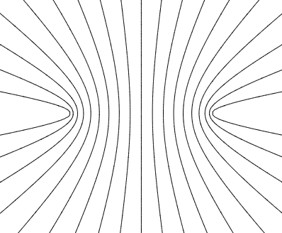
This mapping may be used to solve several electrostatics problems with the geometry shown in Fig. 11a; probably the most surprising of them is the following one. A straight gap of width 2 t is cut in a very thin conducting plane, and voltage V is applied between the resulting half-planes – see the bold straight lines in Fig. 12.
y
V / 2
V / 2
t
t
x
Fig. 2.12. The equipotential surfaces of
the electric field between two thin
conducting semi-planes (or rather their
cross-sections by the plane z = const).
Selecting a Cartesian coordinate system with the z-axis directed along the cut, the y-axis normal to the plane, and the origin in the middle of the cut (Fig. 12), we can write the boundary conditions of this Laplace problem as
V / ,
2
for x t, y
,
0
(2.82)
V / ,
2
for x t, y 0.
(Due to the problem’s symmetry, we may expect that in the middle of the gap, i.e. at – t < x < + t and y =
0, the electric field is parallel to the plane and hence / y = 0.) The comparison of Figs. 11 and 12
shows that if we normalize our coordinates { x, y} to t, Eqs. (81) provide the conformal mapping of our system onto the plane z to a plane capacitor on the plane w, with the voltage V between two conducting planes located at u = 1. Since we already know that in that case = ( V/2) u, we may immediately use the first of Eqs. (81b) to write the final solution of the problem:34
V
V
2 x
1
u sin
.
(2.83)
2
2
2
( x t) y 1/2
2
2
( x t) y 1/2
The thin lines in Fig. 12 show the corresponding equipotential surfaces;35 it is evident that the electric field concentrates at the gap edges, just as it did at the edge of the thin disk (Fig. 8). Let me 34 This result may be also obtained by the Green’s function method, to be discussed in Sec. 10 below.
35 Another graphical representation of the electric field distribution, by field lines, is less convenient. (It is more useful for the magnetic field, which may be represented by a scalar potential only in particular cases, so there is no surprise that the field lines were introduced only by Michael Faraday in the 1830s.) As a reminder, the field Chapter 2
Page 22 of 68
EM: Classical Electrodynamics
leave the remaining calculation of the surface charge distribution and the mutual capacitance between the half-planes (per unit length of the system in the z-direction) for the reader’s exercise.
2.5. Variable separation – Cartesian coordinates
The general approach of the methods discussed in the last two sections was to satisfy the Laplace equation by a function of a single variable that also satisfies the boundary conditions. Unfortunately, in many cases this cannot be done – at least, using reasonably simple functions. In this case, a very powerful method called the variable separation,36 may work, typically producing “semi-analytical”
results in the form of series (infinite sums) of either elementary or well-studied special functions. Its main idea is to look for the solution of the boundary problem (35) as the sum of partial solutions,
c ,
(2.84)
k k
k
where each function k satisfies the Laplace equation, and then select the set of coefficients ck to satisfy the boundary conditions. More specifically, in the variable separation method, the partial solutions k are looked for in the form of a product of functions, each depending on just one spatial coordinate.
Let us discuss this approach on the classical example of a rectangular box with conducting walls (Fig. 13), with the same potential (that I will take for zero) at all its sidewalls and the lower lid, but a different potential V at the top lid ( z = c). Moreover, to demonstrate the power of the variable separation method, let us carry out all the calculations for a more general case when the top lid’s potential is an arbitrary 2D function V( x, y).37
z
c
V ( x, y)
Fig. 2.13. The standard playground for the
0
b
variable separation discussion: a rectangular box
y
0
with five conducting, grounded walls and a fixed
potential distribution V( x, y) on the top lid.
a
x
For this geometry, it is natural to use the Cartesian coordinates { x, y, z}, representing each of the partial solutions in Eq. (84) as the following product
line is the curve to which the field vectors are tangential at each point. Hence the electric field lines are always normal to the equipotential surfaces, so it is always straightforward to sketch them, if desirable, from the equipotential surface pattern – like the one shown in Fig. 12.
36 This method was already discussed in CM Sec. 6.5 and then used also in Secs. 6.6 and 8.4 of that course.
However, it is so important that I need to repeat its discussion in this part of my series, for the benefit of the readers who have skipped the Classical Mechanics course for whatever reason.
37 Such voltage distributions may be implemented in practice, for example, using the so-called mosaic electrodes consisting of many electrically-insulated and individually-biased panels.
Chapter 2
Page 23 of 68
EM: Classical Electrodynamics
X ( x) Y ( y) Z ( z) .
(2.85)
k
Plugging it into the Laplace equation expressed in the Cartesian coordinates,
2
2
2
k
k
k 0 ,
(2.86)
2
2
2
x
y
z
and dividing the result by XYZ, we get
1
2
d X
1 2
d Y
1 2
d Z
0 .
(2.87)
2
2
2
X dx
Y dy
Z dz
Here comes the punch line of the variable separation method: since the first term of this sum may depend only on x, the second one only of y, etc., Eq. (87) may be satisfied everywhere in the volume only if each of these terms equals a constant. In a minute we will see that for our current problem (Fig.
13), these constant x- and y-terms have to be negative; hence let us denote these variable separation constants as (-2) and (-2), respectively. Now Eq. (87) shows that the constant z-term has to be positive; denoting it as 2 we get the following relation:
2
2
2
.
(2.88)
Now the variables are separated in the sense that for the functions X( x), Y( y), and Z( z) we got separate ordinary differential equations,
2
2
2
d X
d Y
d Z
2
X ,
0
2
Y ,
0
2
Z ,
0
(2.89)
2
2
2
dx
dy
dz
which are related only by Eq. (88) for their constant parameters.
Let us start with the equation for X( x). Its general solution is the sum of functions sin x and cos x, multiplied by arbitrary coefficients. Let us select these coefficients to satisfy our boundary conditions. First, since X should vanish at the back vertical wall of the box (i.e., with the coordinate origin choice shown in Fig. 13, at x = 0 for any y and z), the coefficient at cos x should be zero. The remaining coefficient (at sin x) may be included in the general factor ck in Eq. (84), so we may take X
in the form
X sin x .
(2.90)
This solution satisfies the boundary condition at the opposite wall ( x = a) only if the product a is a multiple of , i.e. if is equal to any of the following numbers (commonly called eigenvalues):38
,
n
with n ,
1 ,...
2
(2.91)
n
a
(Terms with negative values of n would not be linearly-independent from those with positive n and may be dropped from the sum (84). The value n = 0 is formally possible but would give X = 0, i.e. k = 0, at 38 Note that according to Eqs. (91)-(92), as the spatial dimensions a and b of the system are increased, the distances between the adjacent eigenvalues tend to zero. This fact implies that for spatially infinite systems, the eigenvalue spectra are continuous, so the sums of the type (84) become integrals; however, the general approach remains the same. A few problems of this type are provided in Sec. 9 for the reader’s exercise.
Chapter 2
Page 24 of 68
EM: Classical Electrodynamics
any x, i.e. no contribution to sum (84), so it may be dropped as well.) Now we see that we indeed had to take real, i.e. 2 positive – otherwise, instead of the oscillating function (90), we would have a sum of two exponential functions, which cannot equal zero at two independent points of the x-axis.
Since the equation (89) for function Y( y) is similar to that for X( x), and the boundary conditions on the walls perpendicular to axis y ( y = 0 and y = b) are similar to those for x-walls, the absolutely similar reasoning gives
Y sin y,
,
m
with m ,
1 ,...
2
,
(2.92)
m
b
where the integer m may be selected independently of n. Now we see that according to Eq. (88), the separation constant depends on two integers n and m, so the relationship may be rewritten as 1/ 2
2
2
n
m
.
(2.93)
nm
2 2
n
m 1/ 2
a
b
The corresponding solution of the differential equation for Z may be represented as a linear combination of two exponents exp{ nmz}, or alternatively of two hyperbolic functions, sinh nmz and cosh nmz, with arbitrary coefficients. At our choice of coordinate origin, the latter option is preferable because cosh nmz cannot satisfy the zero boundary condition at the bottom lid of the box ( z = 0). Hence we may take Z in the form
Z sinh z ,
(2.94)
nm
which automatically satisfies that condition.
Now it is the right time to merge Eqs. (84)-(85) and (90)-(94), replacing the temporary index k with the full set of possible eigenvalues, in our current case of two integer indices n and m: Variable
separation
nx
my
( x, y, z)
in Cartesian
c sin
sin
sinh z ,
(2.95)
nm
n,
1
a
b
nm
m
coordinates
(example) where nm is given by Eq. (93). This solution satisfies not only the Laplace equation but also the boundary conditions on all walls of the box, besides the top lid, for arbitrary coefficients cnm. The only job left is to choose these coefficients from the top-lid requirement:
nx
my
( x, y, c)
c sin
sin
sinh c V ( x, y) .
(2.96)
nm
nm
n, m 1
a
b
It may look bad to have just one equation for the infinite set of coefficients cnm. However, the decisive help comes from the fact that the functions of x and y that participate in Eq. (96), form full, orthogonal sets of 1D functions. The last term means that the integrals of the products of the functions with different integer indices over the region of interest equal zero. Indeed, direct integration gives a
nx
n'x
a
sin
sin
dx ,
(2.97)
a
a
2 nn'
0
where nn’ is the Kronecker symbol, and similarly for y (with the evident replacements a b, and n
m). Hence, a fruitful way to proceed is to multiply both sides of Eq. (96) by the product of the basis functions, with arbitrary indices n’ and m’, and integrate the result over x and y: Chapter 2
Page 25 of 68
EM: Classical Electrodynamics
a
nx
n'x
b
my
m'y
a
b
n'x
m'y
c sinh c sin
sin
dx sin
sin
dy dx dyV ( x, y)sin
sin
. (2.98)
nm
nm
n, m 1
a
a
b
b
a
b
0
0
0
0
Due to Eq. (97), all terms on the left-hand side of the last equation, besides those with n = n’ and m =
m’, vanish, and (replacing n’ with n, and m’ with m, for notation brevity) we finally get a
b
4
nx
my
c
dx dyV ( x, y)sin
sin
.
(2.99)
nm
ab sinh c
a
b
nm
0
0
The relations (93), (95), and (99) give the complete solution of the posed boundary problem; we can see both good and bad news here. The first bit of bad news is that in the general case, we still need to work out the integrals (99) – formally, the infinite number of them. In some cases, it is possible to do this analytically, in one shot. For example, if the top lid in our problem is a single conductor, i.e. has a constant potential V 0, we may take V( x,y) = V 0 = const, and both 1D integrations are elementary; for example
a
nx
a n
a
2 , for
odd,
n
sin
dx
sin d
(2.100)
a
n
n
0
0
for
,
0
even,
n
and similarly for the integral over y, so
16 V
,
1
if
both
n
and
m
odd,
are
c
0
(2.101)
nm
2
nm sinh c
nm
otherwise.
0,
The second bad news is that even on such a happy occasion, we still have to sum up the series (95), so our result may only be called analytical with some reservations because in most cases we need to perform numerical summation to get the final numbers or plots.
Now the first good news. Computers are very efficient for both operations (95) and (99), i.e. for the summation and integration. (As was discussed in Sec. 1.2, random errors are averaged out at these operations.) As an example, Fig. 14 shows the plots of the electrostatic potential in a cubic box ( a = b =
c), with an equipotential top lid ( V = V 0 = const), obtained by a numerical summation of the series (95), using the analytical expression (101). The remarkable feature of this calculation is a very fast convergence of the series; for the middle cross-section of the cubic box ( z/ c = 0.5), already the first term (with n = m = 1) gives an accuracy of about 6%, while the sum of four leading terms (with n, m = 1, 3) reduces the error to just 0.2%. (For a longer box, c > a, b, the convergence is even faster – see the discussion below.) Only very close to the corners between the top lid and the sidewalls, where the potential changes rapidly, several more terms are necessary to get a reasonable accuracy.
The related piece of good news is that our “semi-analytical” result allows its ultimate limits to be explored analytically. For example, Eq. (93) shows that for a very flat box (with c << a, b), n,mz n,mc
<< 1 at least for the lowest terms of series (95), with n, m << c/ a, c/ b. In this case, the sinh functions in Eqs. (96) and (99) may be well approximated with their arguments, and their ratio by z/c. So if we limit the summation to these terms, Eq. (95) gives a very simple result
z
( x, y) V ( x, y) ,
(2.102)
c
Chapter 2
Page 26 of 68
EM: Classical Electrodynamics
which means that each elementary segment of the flat box behaves just as a plane capacitor. Only near the sidewalls, the higher terms in the series (95) are important, producing some deviations from Eq.
(102). (For the general problem with an arbitrary function V( x,y), this is also true in all regions where this function changes sharply.)
y b / 2
y b / 2
z / c 95
.
0
0.8
0.8
0.6
0.6
( ,
x y, z)
75
.
0
V 0
0.4
0.4
x
5
.
0
a
2
.
0
1
.
0
5
.
0
0.2
0.2
05
.
0
25
.
0
0
0
0
0.2
0.4
0.6
0.8
0
0.2
0.4
0.6
0.8
x / a
z / c
Fig. 2.14. The electrostatic potential’s distribution inside a cubic box ( a = b = c) with a constant voltage V 0
on the top lid (Fig. 13), calculated numerically from Eqs. (93), (95), and (101). The dashed line on the left panel shows the contribution of the main term of the series (with n = m = 1) to the full result, for z/ c = 0.5.
In the opposite limit ( a, b << c), Eq. (93) shows that on the contrary, n,mc >> 1 for all n and m.
Moreover, the ratio sinh n,mz/sinh n,mc drops sharply if either n or m is increased, provided that z is not too close to c. Hence in this case a very good approximation may be obtained by keeping just the leading term, with n = m = 1, in Eq. (95), so the challenge of summation disappears. (As was discussed above, this approximation works reasonably well even for a cubic box.) In particular, for the constant potential of the upper lid, we can use Eq. (101) and the exponential asymptotic for both sinh functions, to get a very simple formula:
16
x
y
2 a 2 b1/2
sin
sin
exp
c z .
(2.103)
2
( )
a
b
ab
These results may be readily generalized to some other problems. For example, if all walls of the box shown in Fig. 13 have an arbitrary potential distribution, we may use the linear superposition principle to represent the electrostatic potential distribution as the sum of six partial solutions of the type of Eq. (95), each with one wall biased by the corresponding voltage, and all other grounded ( = 0).
To summarize, the results given by the variable separation method in the Cartesian coordinates are closer to what we could call a genuinely analytical solution than to a purely numerical solution.
Chapter 2
Page 27 of 68
EM: Classical Electrodynamics
Now, let us explore the issues that arise when this method is applied in other orthogonal coordinate systems.
2.6. Variable separation – polar coordinates
If a system of conductors is cylindrical, the potential distribution is independent of the z-
coordinate along the cylinder axis: / z =0, and the Laplace equation becomes two-dimensional. If the conductor’s cross-section is rectangular, the variable separation method works best in Cartesian coordinates { x, y}, and is just a particular case of the 3D solution discussed above. However, if the cross-section is circular, much more compact results may be obtained by using the polar coordinates {,
}. As we already know from Sec. 3(ii), these 2D coordinates are orthogonal, so the two-dimensional Laplace operator is a sum of two separable terms.39 Requiring, just as we have done above, each component of the sum (84) to satisfy the Laplace equation, we get
1
k
1
2
k 0
.
(2.104)
2
2
In a full analogy with Eq. (85), let us represent each particular solution k as a product R() F().
Plugging this expression into Eq. (104) and then dividing all its parts by RF /2, we get
d dR 1 2
d
F 0
.
(2.105)
2
R
d
d F
d
Following the same reasoning as for the Cartesian coordinates, we get two separated ordinary differential equations
d d
R
2
R ,
(2.106)
d
d
2
d
F
2
F ,
0
(2.107)
2
d
where 2 is the variable separation constant.
Let us start their analysis from Eq. (106), plugging into it a probe solution R = c where c and
are some constants. The elementary differentiation shows that if 0, the equation is indeed satisfied for any c, with just one requirement imposed on the constant , namely 2 = 2. This means that the following linear superposition
R
a
b ,
for ,
0
(2.108)
with any constant coefficients a and b, is also a solution of Eq. (106). Moreover, the general theory of linear ordinary differential equations tells us that the solution of a second-order equation like Eq. (106) may only depend on just two constant factors that scale two linearly independent functions. Hence, for all values 2 0, Eq. (108) presents the general solution of that equation. The case when = 0, in which the functions + and – are just constants and hence are not linearly independent, is special, but in this case, the integration of Eq. (106) is straightforward,40 giving
39 See, e.g., MA Eq. (10.3) with / z = 0.
40 Actually, we have already performed it in Sec. 3 – see Eq. (43).
Chapter 2
Page 28 of 68


Essential Graduate Physics
EM: Classical Electrodynamics
R a b ln ,
for 0.
(2.109)
0
0
In order to specify the separation constant, let us explore Eq. (107), whose general solution is
c cos s sin, for 0,
F
(2.110)
c s ,
for
.
0
0
0
There are two possible cases here. In many boundary problems solvable in cylindrical coordinates, the free-space region, in which the Laplace equation is valid, extends continuously around the origin point
= 0. In this region, the potential has to be continuous and uniquely defined, so F has to be a 2-periodic function of . For that, one needs the product ( +2) to equal + 2 n, with n being an integer, immediately giving us a discrete spectrum of possible values of the variable separation constant:
n ,
0 ,
1 ,...
2