Media Processing in Processing by Davide Rocchesso - HTML preview
Download the book in PDF, ePub, Kindle for a complete version.
object along three orthogonal axes, and on the orientation of the plane of projection with respect
to these axes. In particular, in the isometric projection the projections of the axes form angles of 120 ° . The isometric projection has the property that equal segments on the three axes remain
equal when they are projected onto the plane. In order to obtain the isometric projection of an
object whose main axes are parallel to the coordinate axes, we can first rotate the object by
45 ° about the y axis, and then rotate by
about the x axis.
Oblique projection
We can talk about oblique projection every time the projector rays are oblique (non-orthogonal) to
the projection plane. In order to deviate the projector rays from the normal direction by the angles
θ and φ we must use a projection matrix
Casting shadows
As we have seen, Processing has a local illumination model, thus being impossible to cast
shadows directly. However, by manipulating the affine transformation matrices we can cast
shadows onto planes. The method is called flashing in the eye, thus meaning that the optical
center of the scene is moved to the point where the light source is positioned, and then a
perspective transformation is made, with a plane of projection that coincides with the plane where
we want to cast the shadow on.
Example 3.3.
The following program projects on the floor the shadow produced by a light source positioned
on the y axis. The result is shown in Figure 3.2
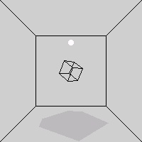
Figure 3.2. Casting a shadow
size(200, 200, P3D);
float centro = 100;
float yp = 70; //floor (plane of projection) distance from center
float yl = 40; //height of light (center of projection) from center
translate(centro, centro, 0); //center the world on the cube
noFill();
box(yp*2); //draw of the room
pushMatrix();
fill(250); noStroke();
translate(0, -yl, 0); // move the virtual light bulb higher
sphere(4); //draw of the light bulb
stroke(10);
popMatrix();
pushMatrix(); //draw of the wireframe cube
noFill();
rotateY(PI/4); rotateX(PI/3);
box(20);
popMatrix();
// SHADOW PROJECTION BY COMPOSITION
// OF THREE TRANSFORMATIONS (the first one in
// the code is the last one to be applied)
translate(0, -yl, 0); // shift of the light source and the floor back
// to their place (see the translation below)
applyMatrix(1, 0, 0, 0,
0, 1, 0, 0,
0, 0, 1, 0,
0, 1/(yp+yl), 0, 0); // projection on the floor
// moved down by yl
translate(0, yl, 0); // shift of the light source to center
// and of the floor down by yl
pushMatrix(); // draw of the cube that generate the shadow
fill(120, 50); // by means of the above transformations
noStroke();
rotateY(PI/4); rotateX(PI/3);
box(20);
popMatrix();
Pills of OpenGL
is a set of functions that allow the programmer to access the graphic system. Technically
speaking, it is an . Its main scope is the graphic rendering of a scene populated by 3D objects and
lights, from a given viewpoint. As far as the programmer is concerned, OpenGL allows to describe
geometric objects and some of their properties, and to decide how such objects have to be
illuminated and seen. As far as the implementation is concerned, OpenGL is based on the graphic
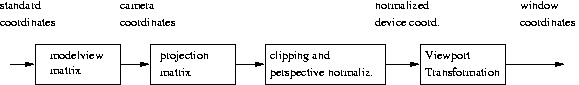
pipeline , made of modules as reported in Figure 3.3. An excellent book on interactive graphics in OpenGL was written by Angel [link].
Figure 3.3. The OpenGL pipeline
In Processing (and in OpenGL), the programmer specifies the objects by means of world
coordinates (standard coordinates). The model-view matrix is the transformation matrix used to
go from standard coordinates to a space associated with the camera. This allows to change the
camera viewpoint and orientation dynamically. In OpenGL this is done with the function
gluLookAt(), which is reproduced in Processing by the camera(). The first triple of
parameters identifies the position, in world coordinates, of the optical center of the camera ( eye
point). The second triple of parameters identifies a point where the camera is looking at ( center
of the scene). The third triple of coordinates identifies a vector aimed at specifying the viewing
vertical. For example, the program
void setup() {
size(100, 100, P3D);
noFill();
frameRate(20);
}
void draw() {
background(204);
camera(70.0, 35.0, 120.0, 50.0, 50.0, 0.0,
(float)mouseX /width, (float)mouseY /height, 0.0);
translate(50, 50, 0);
rotateX(-PI/6);
rotateY(PI/3);
box(45);
}
draws the wireframe of a cube and enables the dynamic rotation of the camera.
The projection matrix is responsible for the projection on the viewing window, and this
projection can be either parallel (orthographic) or perspective. The orthographic projection can be
activated with the call ortho(). The perspective projection is the default one, but it can be
explicitly activated with the call perspective(). Particular projections, such as the oblique
ones, can be obtained by distortion of objects by application of the applyMatrix(). There is
also the texture matrix, but textures are treated in another module.
For each type of matrix, OpenGL keeps a stack, the current matrix being on top. The stack data
structure allows to save the state (by the pushMatrix()) before performing new
transformations, or to remove the current state and activate previous states (by the
popMatrix()). This is reflected in the Processing operations described in The Section Called
“The Stack Of Transformations”. In OpenGL, the transformations are applied according to the
sequence
1. Push on the stack;
2. Apply all desired transformations by multiplying by the stack-top matrix;
3. Draw the object (affected by transformations);
4. Pop from the stack.
A viewport is a rectangular area of the display window. To go from the perspective projection
plane to the viewport two steps are taken: (i) transformation into a 2 x 2 window centered in the
origin ( normalized device coordinates ) (ii) mapping the normalized window onto the viewport.
Using the normalized device coordinates, the clipping operation, that is the elimination of objects
or parts of objects that are not visible through the window, becomes trivial. screenX(),
screenY(), and screenZ() gives the X-Y coordinates produced by the viewport
transformation and by the previous operators in the chain of Figure 3.3.
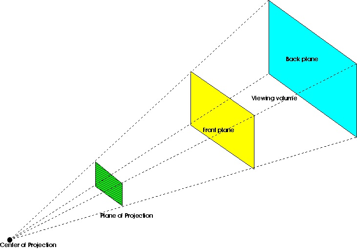
The viewing frustum is the solid angle that encompasses the perspective projection, as shown in
Figure 3.4. The objects (or their parts) belonging to the viewing volume are visualized, the remaining parts are subject to clipping. In Processing (and in OpenGL) the frustum can be defined
by positioning the six planes that define it (frustum()), or by specification of the vertical
angle, the, aspect ratio, and the positions of the front and back planes (perspective()). One
may ask how the system removes the hidden faces, i.e., those faces that are masked by other faces
in the viewing volume. OpenGL uses the algorithm, which is supported by the graphic
accelerators. The board memory stores a 2D memory area (the z-buffer) corresponding to the
pixels of the viewing window, and containing depth values. Before a polygon gets projected on the
viewing window the board checks if the pixels affected by such polygon have a depth value
smaller than the polygon being drawn. If this is the case, it means that there is an object that
masks the polygon.
Figure 3.4. The viewing frustum
Sophisticated geometric transformations are possible by direct manipulation of the projection and
model-view matrices. This is possible, in Processing, starting from the unit matrix, loaded with
resetMatrix(), and proceeding by matrix multiplies done with the applyMatrix().
Run and analyze the Processing code
size(200, 200, P3D);
println("Default matrix:"); printMatrix();
noFill();
ortho(-width/2, width/2, -height/2, height/2, -100, 100);
translate(100, 100, 0);
println("After translation:"); printMatrix();
rotateX(atan(1/sqrt(2)));
println("After about-X rotation:"); printMatrix();
rotateY(PI/4);
println("After about-Y rotation:"); printMatrix();
box(100);
What is visualized and what it the kind of projection used? How do you interpret the matrices
printed out on the console? Can one invert the order of rotations?
The wireframe of a cube is visualized in isometric projection. The latter three matrices represent,
one after the other, the three operations of translation (to center the cube to the window), rotation
about the x axis, and rotation about the y axis. A sequence of two rotations correspond to the product of two rotation matrices, and the outcome is not order independent (product is not
commutative). The product of two rotation matrices RxRy correspond to performing the rotation
about y first, and then the rotation about x .
Write a Processing program that performs the oblique projection of a cube.
For example:
size(200, 200, P3D);
float theta = PI/6;
float phi = PI/12;
noFill();
ortho(-width/2, width/2, -height/2, height/2, -100, 100);
translate(100, 100, 0);
applyMatrix(1, 0, - tan(theta), 0,
0, 1, - tan(phi), 0,
0, 0, 0, 0,
0, 0, 0, 1);
box(100);
Visualize a cube that projects its shadow on the floor, assuming that the light source is at infinite
distance (as it is the case, in practice, for the sun).
We do it similarly to Example 3.3, but the transformation is orthographic:
size(200, 200, P3D);
noFill();
translate(100, 100, 0);
pushMatrix();
rotateY(PI/4); rotateX(PI/3);
box(30);
popMatrix();
translate(0, 60, 0); //cast a shadow from infinity (sun)
applyMatrix(1, 0, 0, 0,
0, 0, 0, 0,
0, 0, 1, 0,
0, 0, 0, 1);
fill(150);
pushMatrix();
noStroke();
rotateY(PI/4); rotateX(PI/3);
box(30);
popMatrix();
References
1. Edward Angel. (2001). Interactive Computer Graphics: A Top-Down Approach With OPENGL
primer package-2nd Edition. Prentice-Hall, Inc.
Glossary
Definition: Spline
Piecewise-polynomial curve, with polynomials connected with continuity at the boldknots See
m11153m11153Introduction to Splines and, for an introduction to the specific kind of splines
(Catmull-Rom) used in Processing, the term in Wikipedia.
Solutions


Chapter 4. Signal Processing in Processing: Sampling
and Quantization
Sampling
Both sounds and images can be considered as signals, in one or two dimensions, respectively.
Sound can be described as a fluctuation of the acoustic pressure in time, while images are spatial
distributions of values of luminance or color, the latter being described in its RGB or HSB
components. Any signal, in order to be processed by numerical computing devices, have to be
reduced to a sequence of discrete samples, and each sample must be represented using a finite
number of bits. The first operation is called sampling, and the second operation is called
quantization of the domain of real numbers.
1-D: Sounds
Sampling is, for one-dimensional signals, the operation that transforms a continuous-time signal
(such as, for instance, the air pressure fluctuation at the entrance of the ear canal) into a discrete-
time signal, that is a sequence of numbers. The discrete-time signal gives the values of the
continuous-time signal read at intervals of T seconds. The reciprocal of the sampling interval is
called sampling rate
. In this module we do not explain the theory of sampling, but we
rather describe its manifestations. For a a more extensive yet accessible treatment, we point to the
Introduction to Sound Processing [link]. For our purposes, the process of sampling a 1-D signal can be reduced to three facts and a theorem.
Fact 1: The Fourier Transform of a discrete-time signal is a function (called spectrum) of the continuous variable ω , and it is periodic with period 2 π . Given a value of ω , the Fourier transform gives back a complex number that can be interpreted as magnitude and phase
(translation in time) of the sinusoidal component at that frequency.
Fact 2: Sampling the continuous-time signal x( t) with interval T we get the discrete-time signal x( n)= x( nT) , which is a function of the discrete variable n .
Fact 3: Sampling a continuous-time signal with sampling rate F s produces a discrete-time
signal whose frequency spectrum is the periodic replication of the original signal, and the
replication period is F s . The Fourier variable ω for functions of discrete variable is converted into the frequency variable f (in Hertz) by means of
.
The Figure 4.1 shows an example of frequency spectrum of a signal sampled with sampling rate F s . In the example, the continuous-time signal had all and only the frequency components
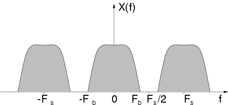

between – F b and F b . The replicas of the original spectrum are sometimes called images.
Figure 4.1. Frequency spectrum of a sampled signal
Given the facts, we can have an intuitive understanding of the Sampling Theorem, historically attributed to the scientists Nyquist and Shannon.
Theorem 4.1.
A continuous-time signal x( t) , whose spectral content is limited to frequencies smaller than
F b (i.e., it is band-limited to F b ) can be recovered from its sampled version x( n) if the sampling rate is larger than twice the bandwidth (i.e., if F s>2 F b )
The reconstruction can only occur by means of a filter that cancels out all spectral images except
for the one directly coming from the original continuous-time signal. In other words, the canceled
images are those having frequency components higher than the Nyquist frequency defined as .
The condition required by the sampling theorem is equivalent to saying that no overlaps between spectral images are allowed. If such superimpositions were present, it wouldn't be possible to
design a filter that eliminates the copies of the original spectrum. In case of overlapping, a filter
that eliminates all frequency components higher than the Nyquist frequency would produce a
signal that is affected by aliasing. The concept of aliasing is well illustrated in the Aliasing
Applet, where a continuous-time sinusoid is subject to sampling. If the frequency of the sinusoid is too high as compared to the sampling rate, we see that the the waveform that is reconstructed
from samples is not the original sinusoid, as it has a much lower frequency. We all have
familiarity with aliasing as it shows up in moving images, for instance when the wagon wheels in
western movies start spinning backward. In that case, the sampling rate is given by the frame
rate, or number of pictures per second, and has to be related with the spinning velocity of the
wheels. This is one of several stroboscopic phenomena.
In the case of sound, in order to become aware of the consequences of the 2 π periodicity of
discrete-time signal spectra (see Figure 4.1) and of violations of the condition of the sampling theorem, we examine a simple case. Let us consider a sound that is generated by a sum of

sinusoids that are harmonics (i.e., integer multiples) of a fundamental. The spectrum of such
sound would display peaks corresponding to the fundamental frequency and to its integer
multiples. Just to give a concrete example, imagine working at the sampling rate of 44100 Hz and
summing 10 sinusoids. From the sampling theorem we know that, in our case, we can represent
without aliasing all frequency components up to 22050 Hz. So, in order to avoid aliasing, the
fundamental frequency should be lower than 2205 Hz. The Processing (with Beads library) code
reported in table Table 4.1 implements a generator of sounds formed by 10 harmonic sinusoids.
To produce such sounds it is necessary to click on a point of the display window. The x coordinate
would vary with the fundamental frequency, and the window will show the spectral peaks
corresponding to the generated harmonics. When we click on a point whose x coordinate is larger
than of the window width, we still see ten spectral peaks. Otherwise, we violate the sampling
theorem and aliasing will enter our representation.
Table 4.1.
import beads.*; // import the beads library
import beads.Buffer;
import beads.BufferFactory;
AudioContext ac;
PowerSpectrum ps;
WavePlayer wavetableSynthesizer;
Glide frequencyGlide;
Envelope gainEnvelope;
Gain synthGain;
int L = 16384; // buffer size
int H = 10; //number of harmonics
float freq = 10.00; // fundamental frequency [Hz]
Buffer dSB;
void setup() {
size(1024,200);
frameRate(20);
ac = new AudioContext(); // initialize AudioContext and create buffer
frequencyGlide = new Glide(ac, 200, 10); // initial freq, and transition time
dSB = new DiscreteSummationBuffer().generateBuffer(L, H, 0.5);
wavetableSynthesizer = new WavePlayer(ac, frequencyGlide, dSB);
gainEnvelope = new Envelope(ac, 0.0); // standard gain control of AudioContext
synthGain = new Gain(ac, 1, gainEnvelope);
synthGain.addInput(wavetableSynthesizer);
ac.out.addInput(synthGain);
// Short-Time Fourier Analysis
ShortFrameSegmenter sfs = new ShortFrameSegmenter(ac);
sfs.addInput(ac.out);
FFT fft = new FFT();
sfs.addListener(fft);
ps = new PowerSpectrum();
fft.addListener(ps);
ac.out.addDependent(sfs);
ac.start(); // start audio processing
gainEnvelope.addSegment(0.8, 50); // attack envelope
}
void mouseReleased(){
println("mouseX = " + mouseX);
}
void draw()
{
background(0);
text("click and move the pointer", 800, 20);
frequencyGlide.setValue(float(mouseX)/width*22050/10); // set the fundamental frequency
// the 10 factor is empirically found
float[] features = ps.getFeatures(); // from Beads analysis library
// It will contain the PowerSpectrum:
// array with the power of 256 spectral bands.
if (features != null) { // if any features are returned
for (int x = 0; x < width; x++){
int featureIndex = (x * features.length) / width;
int barHeight = Math.min((int)(features[featureIndex] * 0.05 *
height), height - 1);
stroke(255);
line(x, height, x, height - barHeight);
}
}
}


public class DiscreteSummationBuffer extends BufferFactory {
public Buffer generateBuffer(int bufferSize) { //Beads generic buffer
return generateBuffer(bufferSize, 10, 0.9f); //default values
}
public Buffer generateBuffer(int bufferSize, int numberOfHarmonics, float amplitude)
{
Buffer b = new Buffer(bufferSize);
double amplitudeCoefficient = amplitude / (2.0 * (double)numberOfHarmonics);
double theta = 0.0;
for (int k = 0; k <= numberOfHarmonics; k++) { //additive synthesis
for (int i = 0; i < b.buf.length; i++) {
b.buf[i] = b.buf[i] + (float)Math.sin(i*2*Math.PI*freq*k/b.buf.length)/20;
}
}