Media Processing in Processing by Davide Rocchesso - HTML preview
Download the book in PDF, ePub, Kindle for a complete version.
{4, 16, 26, 16, 4},
{1, 4, 7, 4, 1} };
for (int i=0; i<5; i++)
for (int j=0; j< 5; j++)
kernel[i][j] = kernel[i][j]/273;
// Convolve the image
for(int y=0; y<height; y++) {
for(int x=0; x<width/2; x++) {
float sum = 0;
for(int k=-n2; k<=n2; k++) {
for(int j=-m2; j<=m2; j++) {
// Reflect x-j to not exceed array boundary
int xp = x-j;
int yp = y-k;
if (xp < 0) {
xp = xp + width;
} else if (x-j >= width) {
xp = xp - width;
}
// Reflect y-k to not exceed array boundary
if (yp < 0) {
yp = yp + height;
} else if (yp >= height) {
yp = yp - height;
}
sum = sum + kernel[j+m2][k+n2] * red(get(xp, yp));
}
}
output[x][y] = int(sum);
}
}
// Display the result of the convolution
// by copying new data into the pixel buffer

loadPixels();
for(int i=0; i<height; i++) {
for(int j=0; j<width/2; j++) {
pixels[i*width + j] = color(output[j][i], output[j][i], output[j][i]);
}
}
updatePixels();
Modify the code of Example 7.1 so that the effects of the averaging filter mask and the are compared. What happens if the central value of the convolution mask is increased further?
Then, try to implement the median filter with a 3×3 cross-shaped mask.
Median filter:
// smoothed_glass
// smoothing filter, adapted from REAS:
// http://www.processing.org/learning/examples/blur.html
size(210, 170);
PImage a; // Declare variable "a" of type PImage
a = loadImage("vetro.jpg"); // Load the images into the program
image(a, 0, 0); // Displays the image from point (0,0)
// corrupt the central strip of the image with random noise
float noiseAmp = 0.1;
loadPixels();
for(int i=0; i<height; i++) {
for(int j=width/4; j<width*3/4; j++) {
int rdm = constrain((int)(noiseAmp*random(-255, 255) +
red(pixels[i*width + j])), 0, 255);
pixels[i*width + j] = color(rdm, rdm, rdm);
}
}
updatePixels();
int[][] output = new int[width][height];
int[] sortedValues = {0, 0, 0, 0, 0};
int grayVal;
// Convolve the image
for(int y=0; y<height; y++) {
for(int x=0; x<width/2; x++) {
int indSort = 0;
for(int k=-1; k<=1; k++) {
for(int j=-1; j<=1; j++) {
// Reflect x-j to not exceed array boundary
int xp = x-j;
int yp = y-k;
if (xp < 0) {
xp = xp + width;
} else if (x-j >= width) {
xp = xp - width;
}
// Reflect y-k to not exceed array boundary
if (yp < 0) {
yp = yp + height;
} else if (yp >= height) {
yp = yp - height;
}
if ((((k != j) && (k != (-j))) ) || (k == 0)) { //cross selection
grayVal = (int)red(get(xp, yp));
indSort = 0;
while (grayVal < sortedValues[indSort]) {indSort++; }
for (int i=4; i>indSort; i--) sortedValues[i] = sortedValues[i-1];
sortedValues[indSort] = grayVal;
}
}
}
output[x][y] = int(sortedValues[2]);
for (int i=0; i< 5; i++) sortedValues[i] = 0;
}
}
// Display the result of the convolution
// by copying new data into the pixel buffer
loadPixels();
for(int i=0; i<height; i++) {
for(int j=0; j<width/2; j++) {
pixels[i*width + j] =
color(output[j][i], output[j][i], output[j][i]);
}
}
updatePixels();
IIR Filters
The filtering operation represented by Equation is a particular case of difference equation, where a sample of output is only function of the input samples. More generally, it is possible to construct
recursive difference equations, where any sample of output is a function of one or more other
output samples.
()
y( n)=0.5 y( n−1)+0.5 x( n)
allows to compute (causally) each sample of the output by only knowing the output at the previous
instant and the input at the same instant. It is easy to realize that by feeding the system
represented by Equation with an impulse, we obtain the infinite-length sequence
y=[0.5, 0.25, 0.125, 0.0625, ...] . For this purpose, filters of this kind are called Infinite Impulse Response (IIR) filters. The order of an IIR filter is equal to the number of past output samples that it has to store for processing, as dictated by the difference equation. Therefore, the filter of
Equation is a first-order filter. For a given filter order, IIR filters allow frequency responses that are steeper than those of FIR filters, but phase distortions are always introduced by IIR filters. In
other words, the different spectral components are delayed by different time amounts. For
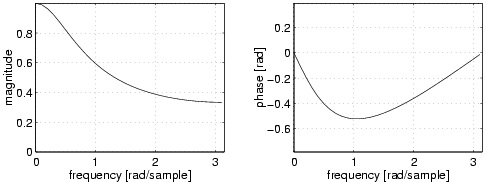
example, Figure 7.6 shows the magnitude and phase responses for the first-order IIR filter represented by the difference equation Equation. Called a the coefficient that weights the dependence on the output previous value ( 0.5 in the specific Equation), the impulse response takes the form h( n)= an . The more a is closer to 1 , the more sustained is the impulse response in time, and the frequency response increases its steepness, thus becoming emphasizing its low-pass
character. Obviously, values of a larger than 1 gives a divergent impulse response and, therefore,
an unstable behavior of the filter.
Figure 7.6. Magnitude and phase response of the IIR first-order filter
IIR filters are widely used for one-dimensional signals, like audio signals, especially for real-time
sample-by-sample processing. Vice versa, it doesn't make much sense to extend recursive
processing onto two dimensions. Therefore, in image processing FIR filters are mostly used.
Resonant filter
In the audio field, second-order IIR filters are particularly important, because they realize an
elementary resonator. Given the difference equation
()
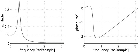
y( n)= a 1 y( n−1)+ a 2 y( n−2)+ b 0 x( n) one can verify that it produces the frequency response of Figure 7.7. The coefficients that gives dependence on the past can be expressed as a 1=2 r cos( ω 0) and a 2=–( r 2) , where ω 0 is the frequency of the resonance peak and r gives peaks that gets narrower when approaching 1 .
Figure 7.7. Magnitude and phase response of the second-order IIR filter
Exercise 4.
Verify that the filtering operation filtra() of the Sound Chooser presented in module Media
Representation in Processing implements an IIR resonant filter. What is the relation between r
and the mouse position along the small bars?
Solutions
Chapter 8. Textures in Processing
Color Interpolation
As seen in Graphic Composition in Processing, one can obtain surfaces as collections of polygons by means of the definition of a vertex within the couple beginShape() -
endShape(). It is possible to assign a color to one or more vertices, in order to make the color
variations continuous ( gradient). For example, you can try to run the code
size(200,200,P3D);
beginShape(TRIANGLE_STRIP);
fill(240, 0, 0); vertex(20,31, 33);
fill(240, 150, 0); vertex(80, 40, 38);
fill(250, 250, 0); vertex(75, 88, 50);
vertex(49, 85, 74);
endShape();
in order to obtain a continuous nuance from red to yellow in the strip of two triangles.
Bilinear Interpolation
The graphical system performs an interpolation of color values assigned to the vertices. This type
of bilinear interpolation is defined in the following way:
For each polygon of the collection
For each side of the polygon one assigns to each point on the segment the color obtained by
means of linear interpolation of the colors of the vertices i e j that define the polygon:
C ij( α)=(1–α) C i+ αC j
A scan line scans the polygon (or, better, its projection on the image window) intersecting at
each step two sides in two points l ed r whose colors have already been identified as C l e C r .
In each point of the scan line the color is determined by linear interpolation
C lr( β)=(1–β) C l+ βC r
A significative example of interpolation of colors associated to the vertices of a cube can be found
in examples of Processing, in the code RGB Cube.
Texture
When modeling a complex scene by means of a composition of simple graphical elements one
cannot go beyond a certain threshold of complexity. Let us think about the example of a
modelization of a natural scene, where one has to represent each single vegetal element, including
the grass of a meadow. It is unconceivable to do this manually. It would be possible to set and
control the grass elements by means of some algorithms. This is an approach taken, for example,
in rendering the hair and skin of characters of the most sophisticated animation movies (see for
example, the Incredibles). Otherwise, especially in case of interactive graphics, one has to resort to using textures. In other words, one employs images that represent the visual texture of the
surfaces and map them on the polygons that model the objects of the scene. In order to have a
qualitative rendering of the surfaces it is necessary to limit the detail level to fragments not
smaller than one pixel and, thus, the texture mapping is inserted in the rendering chain at the
rastering level of the graphic primitives, i.e. where one passes from a 3D geometric description to
the illumination of the pixels on the display. It is at this level that the removal of the hidden
surfaces takes place, since we are interested only in the visible fragments.
In Processing, a texture is defined within a block beginShape() - endShape() by means of
the function texture() that has as unique parameter a variable of type PImage. The following
calls to vertex() can contain, as last couple of parameters, the point of the texture
corresponding to the vertex. In fact, each texture image is parameterized by means of two
variables u and v , that can be referred directly to the line and column of a texel (pixel of a texture) or, alternatively, normalized between 0 and 1 , in such a way that one can ignore the
dimension as well as the width and height of the texture itself. The meaning of the parameters u
and v is established by the command textureMode() with parameter IMAGE or
NORMALIZED.
Example 8.1.
In the code that follows the image representing a broken glass is employed as texture and followed by a color interpolation and the default illumination. The shading of the surfaces,
produced by means of the illumination and the colors, is modulated in a multiplicative way by
the colors of the texture.
size(400,400,P3D);
PImage a = loadImage("vetro.jpg");
lights();
textureMode(NORMALIZED);
beginShape(TRIANGLE_STRIP);
texture(a);
fill(240, 0, 0); vertex(40,61, 63, 0, 0);
fill(240, 150, 0); vertex(340, 80, 76, 0, 1);
fill(250, 250, 0); vertex(150, 176, 100, 1, 1);
vertex(110, 170, 180, 1, 0);
endShape();
Texture mapping
It is evident that the mapping operations from a texture image to an object surface, of arbitrary
shape, implies some form of interpolation. Similarly to what happens for colors, only the vertices
that delimit the surface are mapped onto exact points of the texture image. What happens for the
internal points has to be established in some way. Actually, Processing and OpenGL behave
according to what illustrated in The Section Called “Bilinear Interpolation ”, i.e. by bilinear interpolation: a first linear interpolation over each boundary segment is cascaded by a linear
interpolation on a scan line. If u and v exceed the limits of the texture image, the system
(Processing) can assume that this is repeated periodically and fix it to the values at the border.
A problem that occurs is that a pixel on a display does not necessarly correspond exactly to a
texel. One can map more than one texel on a pixel or, viceversa, a texel can be mapped on several
pixels. The first case corresponds to a downsampling that, as seen in Sampling and
Quantization, can produce aliasing. The effect of aliasing can be attenuated by means of low pass filtering of the texture image. The second case corresponds to upsampling, that in the frequency
domain can be interpreted as increasing the distance between spectral images.
Texture Generation
Textures are not necessarely imported from images, but they can also be generated in an
algorithmic fashion. This is particularly recommended when one wants to generate regular or
pseudo-random patterns. For example, the pattern of a chess-board can be generated by means of
the code
PImage textureImg =
loadImage("vetro.jpg"); // dummy image colorMode(RGB,1);
int biro = 0;
int bbiro = 0;
int scacco = 5;
for (int i=0; i<textureImg.width; i+=scacco) {
bbiro = (bbiro + 1)%2; biro = bbiro;
for (int j=0; j<textureImg.height; j+=scacco) {
for (int r=0; r<scacco; r++)
for (int s=0; s<scacco; s++)
textureImg.set(i+r,j+s, color(biro));
biro = (biro + 1)%2;
}
}
image(textureImg, 0, 0);
The use of the function random, combined with filters of various type, allows a wide flexibility in
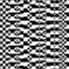
the production of textures. For example, the pattern represented in Figure 8.1 was obtained from a modification of the code generating the chess-board. In particular, we added the line
scacco=floor(2+random(5)); within the outer for, and applied an averaging filter.
Figure 8.1. Algorithmically-generated pattern
How could one modify the code Example 8.1 in order to make the breaks in the glass more evident?
It is sufficient to consider only a piece of the texture, with calls of the type vertex(150,
176, 0.3, 0.3);
Exercise 2.
The excercise consists in modifying the code of the generator of the chess-board in The Section
Called “Texture Generation” in order to generate the texture Figure 8.1.
Exercise 3.
This exercise consists in running and analyzing the following code. Try then to vary the
dimensions of the small squares and the filtering type.
size(200, 100, P3D);
PImage textureImg = loadImage("vetro.jpg"); // dummy image
colorMode(RGB,1);
int biro = 0;
int bbiro = 0;
int scacco = 5;
for (int i=0; i<textureImg.width; i+=scacco) {
// scacco=floor(2+random(5));
bbiro = (bbiro + 1)%2; biro = bbiro;
for (int j=0; j<textureImg.height; j+=scacco) {
for (int r=0; r<scacco; r++)
for (int s=0; s<scacco; s++)
textureImg.set(i+r,j+s, color(biro));
biro = (biro + 1)%2;
}
}
image(textureImg, 0, 0);
textureMode(NORMALIZED);
beginShape(QUADS);
texture(textureImg);
vertex(20, 20, 0, 0);
vertex(80, 25, 0, 0.5);
vertex(90, 90, 0.5, 0.5);
vertex(20, 80, 0.5, 0);
endShape();
// ------ filtering -------
PImage tImg = loadImage("vetro.jpg"); // dummy image
float val = 1.0/9.0;
float[][] kernel = { {val, val, val},
{val, val, val},
{val, val, val} };
int n2 = 1;
int m2 = 1;
colorMode(RGB,255);
// Convolve the image
for(int y=0; y<textureImg.height; y++) {
for(int x=0; x<textureImg.width/2; x++) {
float sum = 0;
for(int k=-n2; k<=n2; k++) {
for(int j=-m2; j<=m2; j++) {
// Reflect x-j to not exceed array boundary
int xp = x-j;
int yp = y-k;
if (xp < 0) {
xp = xp + textureImg.width;
} else if (x-j >= textureImg.width) {
xp = xp - textureImg.width;
}
// Reflect y-k to not exceed array boundary
if (yp < 0) {
yp = yp + textureImg.height;
} else if (yp >= textureImg.height) {
yp = yp - textureImg.height;
}
sum = sum + kernel[j+m2][k+n2] * red(textureImg.get(xp, yp));
}
}
tImg.set(x,y, color(int(sum)));
}
}
translate(100, 0);
beginShape(QUADS);
texture(tImg);
vertex(20, 20, 0, 0);
vertex(80, 25, 0, 0.5);
vertex(90, 90, 0.5, 0.5);
vertex(20, 80, 0.5, 0);
endShape();
Solutions


Chapter 9. Signal Processing in Processing: Miscellanea
Economic Color Representations
In Media Representation in Processing we saw how one devotes 8 bits to each channel corresponding to a primary color. If we add to these the alpha channel, the total number of bits per
pixel becomes 32 . We do not always have the possibility to use such a big amount of memory for
colors. Therefore, one has to adopt various strategies in order to reduce the number of bits per
pixel.
Palette
A first solution comes from the observation that usually in an image, not all of the
224 representable colors are present at the same time. Supposing that the number of colors
necessary for an ordinary image is not greater than 256 , one can think about memorizing the
codes of the colors in a table ( palette), whose elements are accessible by means of an index of
only 8 bits. Thus, the image will require a memory space of 8 bits per pixel plus the space
necessary for the palette. For examples and further explanations see color depth in Wikipedia.
Dithering
Alternatively, in order to have a low number of bits per pixel, one can apply a digital processing
technique called dithering. The idea is that of obtaining a mixture of colors in a perceptual way,
exploiting the proximity of small points of different color. An exhaustive presentation of the
phenomenon can be found at the voice dithering of Wikipedia.
Floyd-Steinberg's Dithering
The Floyd-Steinberg's algorithm is one of the most popular techniques for the distribution of
colored pixels in order to obtain a dithering effect. The idea is to minimize the visual artifacts by
processing the error-diffusion. The algorithm can be resumed as follows:
While proceeding top down and from left to right for each considered pixel,
calculate the difference between the goal color and the closest representable color (error)
spread the error on the contiguous pixels according to the mask
. That is, add of
the error to the pixel on the right of the considered one, add of the error to the pixel
bottom left with respect to the considered one, and so on.

By means of this algorithm it is possible to reproduce an image with different gray levels by
means of a device able to define only white and black points. The mask of the Floyd-Steinberg's
algorithm was chosen in a way that a uniform distribution of gray intensities produces a
chessboard layout pattern.
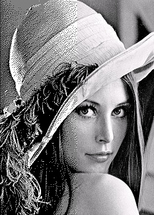
By means of Processing, implement a program to process the file lena, a "dithered" black and white version of the famous Lena image. The image, treated only in the left half, should result similar to that of Figure 9.0
Figure 9.0.
size(300, 420);
PImage a; // Declare variable "a" of type PImage
a = loadImage("lena.jpg"); // Load the images into the program
image(a, 0, 0); // Displays the image from point (0,0)
int[][] output = new int[width][height];
for (int i=0; i<width; i++)
for (int j=0; j<height; j++) {
output[i][j] = (int)red(get(i, j));
}
int grayVal;
float errore;
float val = 1.0/16.0;
float[][] kernel = { {0, 0, 0},
{0, -1, 7*val},
{3*val, 5*val, val }};
for(int y=0; y<height; y++) {
for(int x=0; x<widt