Intro to Digital Signal Processing by Robert Nowak, et al - HTML preview
Download the book in PDF, ePub for a complete version.
will also need to take into account the choice of time.
Stationarity
Below we will now look at a more in depth and mathematical definition of a stationary process.
As was mentioned previously, various levels of stationarity exist and we will look at the most
common types.
First-Order Stationary Process
A random process is classified as first-order stationary if its first-order probability density
function remains equal regardless of any shift in time to its time origin. If we let xt represent a
1
given value at time t 1 , then we define a first-order stationary as one that satisfies the following
equation:
()
fx( xt )= f
1
x( x t 1 + τ )
The physical significance of this equation is that our density function, fx( xt ) , is completely
1
independent of t 1 and thus any time shift, τ.
The most important result of this statement, and the identifying characteristic of any first-order
stationary process, is the fact that the mean is a constant, independent of any time shift. Below we
show the results for a random process, X, that is a discrete-time signal, x[ n] .
()


Second-Order and Strict-Sense Stationary Process
A random process is classified as second-order stationary if its second-order probability density
function does not vary over any time shift applied to both values. In other words, for values xt and
1
xt then we will have the following be equal for an arbitrary time shift τ.
2
()
fx( xt , x )= f
1
t 2
x( x t 1 + τ , x t 2 + τ )
From this equation we see that the absolute time does not affect our functions, rather it only really
depends on the time difference between the two variables. Looked at another way, this equation
can be described as
()
Pr[ X( t 1)≤ x 1, X( t 2)≤ x 2]=Pr[ X( t 1+ τ)≤ x 1, X( t 2+ τ)≤ x 2]
These random processes are often referred to as strict sense stationary (SSS) when all of the
distribution functions of the process are unchanged regardless of the time shift applied to them.
For a second-order stationary process, we need to look at the autocorrelation function to see its most important property. Since we have already stated that a second-order stationary process
depends only on the time difference, then all of these types of processes have the following
property:
()
Wide-Sense Stationary Process
As you begin to work with random processes, it will become evident that the strict requirements
of a SSS process is more than is often necessary in order to adequately approximate our
calculations on random processes. We define a final type of stationarity, referred to as wide-sense
stationary (WSS), to have slightly more relaxed requirements but ones that are still enough to
provide us with adequate results. In order to be WSS a random process only needs to meet the
following two requirements.
1.
2. E[ X( t+ τ)]= Rxx( τ)
Note that a second-order (or SSS) stationary process will always be WSS; however, the reverse
will not always hold true.
2.5. Random Processes: Mean and Variance*


2.5. Random Processes: Mean and Variance*
In order to study the characteristics of a random process, let us look at some of the basic properties and operations of a random process. Below we will focus on the operations of the
random signals that compose our random processes. We will denote our random process with X
and a random variable from a random process or signal by x.
Mean Value
Finding the average value of a set of random signals or random variables is probably the most
fundamental concepts we use in evaluating random processes through any sort of statistical
method. The mean of a random process is the average of all realizations of that process. In
order to find this average, we must look at a random signal over a range of time (possible values)
and determine our average from this set of values. The mean, or average, of a random process,
x( t) , is given by the following equation:
()
This equation may seem quite cluttered at first glance, but we want to introduce you to the various
notations used to represent the mean of a random signal or process. Throughout texts and other
readings, remember that these will all equal the same thing. The symbol, μx( t) , and the X with a bar over it are often used as a short-hand to represent an average, so you might see it in certain
textbooks. The other important notation used is, E[ X] , which represents the "expected value of X"
or the mathematical expectation. This notation is very common and will appear again.
If the random variables, which make up our random process, are discrete or quantized values, such
as in a binary process, then the integrals become summations over all the possible values of the
random variable. In this case, our expected value becomes
()
If we have two random signals or variables, their averages can reveal how the two signals interact.
If the product of the two individual averages of both signals do not equal the average of the
product of the two signals, then the two signals are said to be linearly independent, also referred
to as uncorrelated.
In the case where we have a random process in which only one sample can be viewed at a time,
then we will often not have all the information available to calculate the mean using the density

function as shown above. In this case we must estimate the mean through the time-average mean,
discussed later. For fields such as signal processing that deal mainly with discrete signals and
values, then these are the averages most commonly used.
Properties of the Mean
The expected value of a constant, α , is the constant:
()
E[ α]= α
Adding a constant, α , to each term increases the expected value by that constant:
()
E[ X+ α]= E[ X]+ α
Multiplying the random variable by a constant, α , multiplies the expected value by that
constant.
()
E[ αX]= αE[ X]
The expected value of the sum of two or more random variables, is the sum of each individual
expected value.
()
E[ X+ Y]= E[ X]+ E[ Y]
Mean-Square Value
If we look at the second moment of the term (we now look at x 2 in the integral), then we will have the mean-square value of our random process. As you would expect, this is written as
()
This equation is also often referred to as the average power of a process or signal.
Variance
Now that we have an idea about the average value or values that a random process takes, we are
often interested in seeing just how spread out the different random values might be. To do this, we
look at the variance which is a measure of this spread. The variance, often denoted by σ 2 , is
written as follows:


()
Using the rules for the expected value, we can rewrite this formula as the following form, which is
commonly seen:
()
Standard Deviation
Another common statistical tool is the standard deviation. Once you know how to calculate the
variance, the standard deviation is simply the square root of the variance, or σ .
Properties of Variance
The variance of a constant, α , equals zero:
()
Adding a constant, α , to a random variable does not affect the variance because the mean
increases by the same value:
()
Multiplying the random variable by a constant, α , increases the variance by the square of the
constant:
()
The variance of the sum of two random variables only equals the sum of the variances if the
variable are independent.
()
Otherwise, if the random variable are not independent, then we must also include the
covariance of the product of the variables as follows:
()
Var( X+ Y)= σ( X)2+2Cov( X, Y)+ σ( Y)2


Time Averages
In the case where we can not view the entire ensemble of the random process, we must use time
averages to estimate the values of the mean and variance for the process. Generally, this will only
give us acceptable results for independent and ergodic processes, meaning those processes in
which each signal or member of the process seems to have the same statistical behavior as the
entire process. The time averages will also only be taken over a finite interval since we will only
be able to see a finite part of the sample.
Estimating the Mean
For the ergodic random process, x( t) , we will estimate the mean using the time averaging function defined as
()
However, for most real-world situations we will be dealing with discrete values in our
computations and signals. We will represent this mean as
()
Estimating the Variance
Once the mean of our random process has been estimated then we can simply use those values in
the following variance equation (introduced in one of the above sections)
()
Example
Let us now look at how some of the formulas and concepts above apply to a simple example. We
will just look at a single, continuous random variable for this example, but the calculations and
methods are the same for a random process. For this example, we will consider a random variable
having the probability density function described below and shown in Figure 2.10.
()
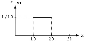


Figure 2.10. Probability Density Function
A uniform probability density function.
First, we will use Equation to solve for the mean value.
()
Using Equation we can obtain the mean-square value for the above density function.
()
And finally, let us solve for the variance of this function.
()
2.6. Correlation and Covariance of a Random Signal*
When we take the expected value, or average, of a random process, we measure several important characteristics about how the process behaves in general. This proves to be a very
important observation. However, suppose we have several random processes measuring different
aspects of a system. The relationship between these different processes will also be an important
observation. The covariance and correlation are two important tools in finding these relationships.


Below we will go into more details as to what these words mean and how these tools are helpful.
Note that much of the following discussions refer to just random variables, but keep in mind that
these variables can represent random signals or random processes.
Covariance
To begin with, when dealing with more than one random process, it should be obvious that it
would be nice to be able to have a number that could quickly give us an idea of how similar the
processes are. To do this, we use the covariance, which is analogous to the variance of a single
variable.
Definition: Covariance
A measure of how much the deviations of two or more variables or processes match.
For two processes, X and Y , if they are not closely related then the covariance will be small, and if they are similar then the covariance will be large. Let us clarify this statement by describing
what we mean by "related" and "similar." Two processes are "closely related" if their distribution spreads are almost equal and they are around the same, or a very slightly different, mean.
Mathematically, covariance is often written as σxy and is defined as
()
This can also be reduced and rewritten in the following two forms:
()
()
Useful Properties
If X and Y are independent and uncorrelated or one of them has zero mean value, then σxy=0
If X and Y are orthogonal, then σxy=–( E[ X] E[ Y])
The covariance is symmetric cov( X, Y)=cov( Y, X)
Basic covariance identity cov( X+ Y, Z)=cov( X, Z)+cov( Y, Z)
Covariance of equal variables cov( X, X)=Var( X)


Correlation
For anyone who has any kind of statistical background, you should be able to see that the idea of
dependence/independence among variables and signals plays an important role when dealing with
random processes. Because of this, the correlation of two variables provides us with a measure of
how the two variables affect one another.
Definition: Correlation
A measure of how much one random variable depends upon the other.
This measure of association between the variables will provide us with a clue as to how well the
value of one variable can be predicted from the value of the other. The correlation is equal to the
average of the product of two random variables and is defined as
()
Correlation Coefficient
It is often useful to express the correlation of random variables with a range of numbers, like a
percentage. For a given set of variables, we use the correlation coefficient to give us the linear
relationship between our variables. The correlation coefficient of two variables is defined in terms
of their covariance and standard deviations, denoted by σx , as seen below ()
where we will always have -1≤ ρ≤1 This provides us with a quick and easy way to view the
correlation between our variables. If there is no relationship between the variables then the
correlation coefficient will be zero and if there is a perfect positive match it will be one. If there is
a perfect inverse relationship, where one set of variables increases while the other decreases, then
the correlation coefficient will be negative one. This type of correlation is often referred to more
specifically as the Pearson's Correlation Coefficient,or Pearson's Product Moment Correlation.
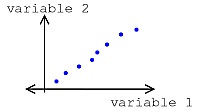
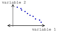
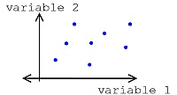
(a) Positive Correlation
(b) Negative Correlation
(c) Uncorrelated (No Correlation)
Figure 2.11.
Types of Correlation


So far we have dealt with correlation simply as a number relating the relationship between any
two variables. However, since our goal will be to relate random processes to each other, which
deals with signals as a function of time, we will want to continue this study by looking at
Example
Now let us take just a second to look at a simple example that involves calculating the covariance
and correlation of two sets of random numbers. We are given the following data sets:
To
begin with, for the covariance we will need to find the expected value, or mean, of x and y.
Next we will solve for the
standard deviations of our two sets using the formula below (for a review click here).
Now we can
finally calculate the covariance using one of the two formulas found above. Since we calculated
the three means, we will use that formula since it will be much simpler.
σxy=10−3.4×3.2=-0.88 And for our last calculation, we will solve for the correlation coefficient,
ρ.
Matlab Code for Example
The above example can be easily calculated using Matlab. Below I have included the code to find
all of the values above.
x = [3 1 6 3 4];
y = [1 5 3 4 3];
mx = mean(x)
my = mean(y)
mxy = mean(x.*y)
% Standard Dev. from built-in Matlab Functions
std(x,1)
std(y,1)
% Standard Dev. from Equation Above (same result as std(?,1))
sqrt( 1/5 * sum((x-mx).^2))
sqrt( 1/5 * sum((y-my).^2))
cov(x,y,1)
corrcoef(x,y)
2.7. Autocorrelation of Random Processes*
Before diving into a more complex statistical analysis of random signals and processes, let us quickly review the idea of correlation. Recall that the correlation of two signals or variables is the expected value of the product of those two variables. Since our focus will be to discover more
about a random process, a collection of random signals, then imagine us dealing with two samples
of a random process, where each sample is taken at a different point in time. Also recall that the
key property of these random processes is that they are now functions of time; imagine them as a
collection of signals. The expected value of the product of these two variables (or samples) will now depend on how quickly they change in regards to time. For example, if the two variables are
taken from almost the same time period, then we should expect them to have a high correlation.
We will now look at a correlation function that relates a pair of random variables from the same
process to the time separations between them, where the argument to this correlation function will
be the time difference. For the correlation of signals