Intro to Digital Signal Processing by Robert Nowak, et al - HTML preview
Download the book in PDF, ePub for a complete version.


()
Now we can plot this result (Figure 1.66):
Figure 1.66.
The sequence from 0 to 4 (the underlined part of the sequence) is the regular convolution result. From this illustration we can see that it is 5-periodic!
General Result
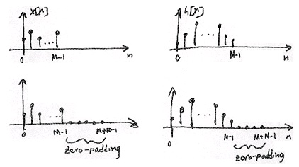
We can compute the regular convolution result of a convolution of an M-point signal x[ n] with an N-point signal h[ n] by padding each signal with zeros to obtain two M+ N−1 length sequences and computing the circular convolution (or equivalently computing the IDFT of
H[ k] X[ k] , the product of the DFTs of the zero-padded signals) (Figure 1.67).
Figure 1.67.
Note that the lower two images are simply the top images that have been zero-padded.
DSP System
Figure 1.68.
The system has a length N impulse response, h[ n]


1. Sample finite duration continuous-time input x( t) to get x[ n] where n={0, …, M−1} .
2. Zero-pad x[ n] and h[ n] to length M+ N−1 .
3. Compute DFTs X[ k] and H[ k]
4. Compute IDFTs of X[ k] H[ k]
where n={0, …, M+ N−1} .
5. Reconstruct y( t)
1.12. Ideal Reconstruction of Sampled Signals*
Reconstruction of Sampled Signals
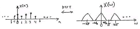
How do we go from x[ n] to CT (Figure 1.69)?
Figure 1.69.
Step 1
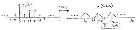
Place x[ n] into CT on an impulse train s( t) (Figure 1.70).
()
Figure 1.70.
Step 2
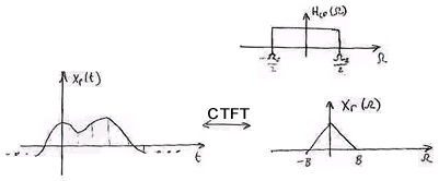


Pass xs( t) through an idea lowpass filter H LP( Ω) (Figure 1.71).
Figure 1.71.
If we had no aliasing then xr[ t]= xc( t) , where x[ n]= xc( nT) .
Ideal Reconstruction System
Figure 1.72.
In Frequency Domain:
1. Xs( Ω)= X( ΩT) where X( ΩT) is the DTFT of x[ n] at digital frequency ω= ΩT .
2. Xr( Ω)= H LP( Ω) Xs( Ω)
Result
Xr( Ω)= H LP( Ω) X( ΩT)
In Time Domain:
1.
2.
Result
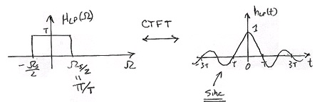

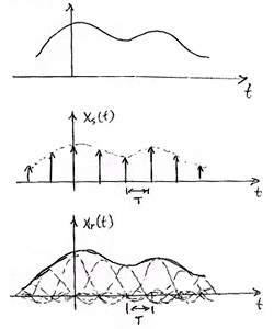

Figure 1.73.
()
h LP( t) "interpolates" the values of x[ n] to generate xr( t) (Figure 1.74).
Figure 1.74.
(1.5)
Sinc Interpolator
1.13. Amplitude Quantization*
The Sampling Theorem says that if we sample a bandlimited signal s( t) fast enough, it can be
recovered without error from its samples s( nTs) , n∈{ …, -1, 0, 1, …} . Sampling is only the first phase of acquiring data into a computer: Computational processing further requires that the


samples be quantized: analog values are converted into digital form. In short, we will have performed analog-to-digital (A/D) conversion.
(a)
(b)
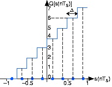
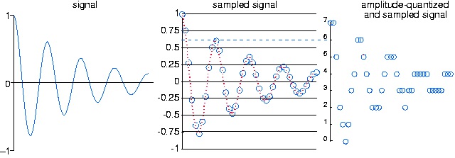
Figure 1.75.
A three-bit A/D converter assigns voltage in the range [-1, 1] to one of eight integers between 0 and 7. For example, all inputs having values lying between 0.5 and 0.75 are assigned the integer value six and, upon conversion back to an analog value, they all become 0.625. The width of a single quantization interval Δ equals
. The bottom panel shows a signal going through the analog-to-digital,
where B is the number of bits used in the A/D conversion process (3 in the case depicted here). First it is sampled, then amplitude-quantized to three bits. Note how the sampled signal waveform becomes distorted after amplitude quantization. For example the two signal values between 0.5 and 0.75 become 0.625. This distortion is irreversible; it can be reduced (but not eliminated) by using more bits in the A/D converter.
A phenomenon reminiscent of the errors incurred in representing numbers on a computer prevents
signal amplitudes from being converted with no error into a binary number representation. In
analog-to-digital conversion, the signal is assumed to lie within a predefined range. Assuming we
can scale the signal without affecting the information it expresses, we'll define this range to be
[–1, 1] . Furthermore, the A/D converter assigns amplitude values in this range to a set of integers.
A B -bit converter produces one of the integers {0, 1, …, 2 B−1} for each sampled input.
Figure 1.75 shows how a three-bit A/D converter assigns input values to the integers. We define a quantization interval to be the range of values assigned to the same integer. Thus, for our
example three-bit A/D converter, the quantization interval Δ is 0.25 ; in general, it is
.


Recalling the plot of average daily highs in this frequency domain problem, why is this plot so jagged? Interpret this effect in terms of analog-to-digital conversion.
The plotted temperatures were quantized to the nearest degree. Thus, the high temperature's
amplitude was quantized as a form of A/D conversion.
Because values lying anywhere within a quantization interval are assigned the same value for
computer processing, the original amplitude value cannot be recovered without error.
Typically, the D/A converter, the device that converts integers to amplitudes, assigns an amplitude
equal to the value lying halfway in the quantization interval. The integer 6 would be assigned to
the amplitude 0.625 in this scheme. The error introduced by converting a signal from analog to
digital form by sampling and amplitude quantization then back again would be half the
quantization interval for each amplitude value. Thus, the so-called A/D error equals half the width
of a quantization interval:
. As we have fixed the input-amplitude range, the more bits available
in the A/D converter, the smaller the quantization error.
To analyze the amplitude quantization error more deeply, we need to compute the signal-to-noise
ratio, which equals the ratio of the signal power and the quantization error power. Assuming the
signal is a sinusoid, the signal power is the square of the rms amplitude:
. The
illustration details a single quantization interval.
Figure 1.76.
A single quantization interval is shown, along with a typical signal's value before amplitude quantization s( nTs) and after Q( s( nTs)) .
ε denotes the error thus incurred.
Its width is Δ and the quantization error is denoted by ε. To find the power in the quantization
error, we note that no matter into which quantization interval the signal's value falls, the error will
have the same characteristics. To calculate the rms value, we must square the error and average it
over the interval.
()
Since the quantization interval width for a B-bit converter equals
, we find that the
signal-to-noise ratio for the analog-to-digital conversion process equals


()
Thus, every bit increase in the A/D converter yields a 6 dB increase in the signal-to-noise ratio.
The constant term 10log101.5 equals 1.76.
This derivation assumed the signal's amplitude lay in the range [-1, 1] . What would the amplitude
quantization signal-to-noise ratio be if it lay in the range [– A, A] ?
The signal-to-noise ratio does not depend on the signal amplitude. With an A/D range of [– A, A] ,
the quantization interval
and the signal's rms value (again assuming it is a sinusoid) is .
How many bits would be required in the A/D converter to ensure that the maximum amplitude
quantization error was less than 60 db smaller than the signal's peak value?
Solving 2– B=.001 results in B=10 bits.
Music on a CD is stored to 16-bit accuracy. To what signal-to-noise ratio does this correspond?
A 16-bit A/D converter yields a SNR of 6×16+10log101.5=97.8 dB.
Once we have acquired signals with an A/D converter, we can process them using digital hardware
or software. It can be shown that if the computer processing is linear, the result of sampling,
computer processing, and unsampling is equivalent to some analog linear system. Why go to all
the bother if the same function can be accomplished using analog techniques? Knowing when
digital processing excels and when it does not is an important issue.
1.14. Classic Fourier Series*
The classic Fourier series as derived originally expressed a periodic signal (period T) in terms of
harmonically related sines and cosines.


()
The complex Fourier series and the sine-cosine series are identical, each representing a signal's
spectrum. The Fourier coefficients, ak and bk , express the real and imaginary parts respectively of the spectrum while the coefficients ck of the complex Fourier series express the spectrum as a
magnitude and phase. Equating the classic Fourier series to the complex Fourier series, an extra factor of two and complex conjugate become necessary to relate the Fourier coefficients in each.
Derive this relationship between the coefficients of the two Fourier series.
Write the coefficients of the complex Fourier series in Cartesian form as ck= Ak+ ⅈBk and
substitute into the expression for the complex Fourier series.
Simplifying each term in the sum using Euler's formula,
We now combine terms that have the same
frequency index in magnitude. Because the signal is real-valued, the coefficients of the complex
Fourier series have conjugate symmetry:
or A– k= Ak and B– k=– Bk . After we add the
positive-indexed and negative-indexed terms, each term in the Fourier series becomes
. To obtain the classic Fourier series, we must have 2 Ak= ak and 2 Bk=– bk .
Just as with the complex Fourier series, we can find the Fourier coefficients using the
orthogonality properties of sinusoids. Note that the cosine and sine of harmonically related
frequencies, even the same frequency, are orthogonal.
()
These
orthogonality relations follow from the following important trigonometric identities.
()
These identities allow you to substitute a sum of sines and/or cosines for a product of them. Each
term in the sum can be integrating by noticing one of two important properties of sinusoids.


The integral of a sinusoid over an integer number of periods equals zero.
The integral of the square of a unit-amplitude sinusoid over a period T equals .
To use these, let's, for example, multiply the Fourier series for a signal by the cosine of the
l th harmonic
and integrate. The idea is that, because integration is linear, the integration
will sift out all but the term involving al .
()
The first and third terms are zero; in the second, the only non-zero term in the sum results when
the indices k and l are equal (but not zero), in which case we obtain
. If k=0= l , we obtain a 0 T .
Consequently,
All of the Fourier coefficients can be found similarly.
()
The expression for a 0 is referred to as the average value of s( t) . Why?
The average of a set of numbers is the sum divided by the number of terms. Viewing signal
integration as the limit of a Riemann sum, the integral corresponds to the average.
What is the Fourier series for a unit-amplitude square wave?
We found that the complex Fourier series coefficients are given by
. The coefficients are
pure imaginary, which means ak=0 . The coefficients of the sine terms are given by
bk=–(2Im( ck)) so that
Thus, the Fourier series for the square wave is
()
Example 1.13.
Let's find the Fourier series representation for the half-wave rectified sinusoid.


()
Begin with the sine terms in the series; to find bk we must calculate the integral
()
Using our trigonometric identities turns our integral of a product of sinusoids into a sum of
integrals of individual sinusoids, which are much easier to evaluate.
()
Thus,
b 2= b 3= …=0
On to the cosine terms. The average value, which corresponds to a 0 , equals . The remainder
of the cosine coefficients are easy to find, but yield the complicated result
()
Thus, the Fourier series for the half-wave rectified sinusoid has non-zero terms for the
average, the fundamental, and the even harmonics.
Glossary
Definition: FFT
(Fast Fourier Transform) An efficient computational algorithm for computing the
m10249m102493DFT.
Solutions
Chapter 2. Random Signals
2.1. Introduction to Random Signals and Processes*
Before now, you have probably dealt strictly with the theory behind signals and systems, as well
as look at some the basic characteristics of signals and systems. In doing so you have developed an important foundation; however, most electrical engineers do not get to work in this type of
fantasy world. In many cases the signals of interest are very complex due to the randomness of the
world around them, which leaves them noisy and often corrupted. This often causes the
information contained in the signal to be hidden and distorted. For this reason, it is important to
understand these random signals and how to recover the necessary information.
Signals: Deterministic vs. Stochastic
For this study of signals and systems, we will divide signals into two groups: those that have a
fixed behavior and those that change randomly. As most of you have probably already dealt with
the first type, we will focus on introducing you to random signals. Also, note that we will be
dealing strictly with discrete-time signals since they are the signals we deal with in DSP and most
real-world computations, but these same ideas apply to continuous-time signals.
Deterministic Signals
Most introductions to signals and systems deal strictly with deterministic signals. Each value of
these signals are fixed and can be determined by a mathematical expression, rule, or table.
Because of this, future values of any deterministic signal can be calculated from past values. For
this reason, these signals are relatively easy to analyze as they do not change, and we can make
accurate assumptions about their past and future behavior.
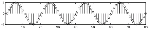
Figure 2.1. Deterministic Signal
An example of a deterministic signal, the sine wave.
Stochastic Signals
Unlike deterministic signals, stochastic signals, or random signals, are not so nice. Random
signals cannot be characterized by a simple, well-defined mathematical equation and their future
values cannot be predicted. Rather, we must use probability and statistics to analyze their
behavior. Also, because of their randomness, average values from a collection of signals are usually studied rather than analyzing one individual signal.
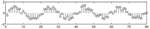
Figure 2.2. Random Signal
We have taken the above sine wave and added random noise to it to come up with a noisy, or random, signal. These are the types of signals that we wish to learn how to deal with so that we can recover the original sine wave.
Random Process
As mentioned above, in order to study random signals, we want to look at a collection of these
signals rather than just one instance of that signal. This collection of signals is called a random
process