Intro to Digital Signal Processing by Robert Nowak, et al - HTML preview
Download the book in PDF, ePub for a complete version.
Intro to Digital Signal Processing
Collection edited by: Robert Nowak
Content authors: Robert Nowak, Don Johnson, Michael Haag, Behnaam Aazhang, Nick
Kingsbury, Benjamin Fite, Melissa Selik, Richard Baraniuk, Dan Calderon, Ivan Selesnick, Bill
Wilson, Hyeokho Choi, Douglas Jones, Swaroop Appadwedula, Matthew Berry, Mark Haun, Dima
Moussa, Daniel Sachs, Roy Ha, Justin Romberg, and Phil Schniter
Online: < http://cnx.org/content/col10203/1.4>
This selection and arrangement of content as a collection is copyrighted by Robert Nowak.
It is licensed under the Creative Commons Attribution License: http://creativecommons.org/licenses/by/1.0
Collection structure revised: 2004/01/22
For copyright and attribution information for the modules contained in this collection, see the " Attributions" section at the end of the collection.
Intro to Digital Signal Processing
Table of Contents
1.2. Digital Image Processing Basics
Linear Shift Invariant Systems
1.5. DFT as a Matrix Operation
Representing DFT as Matrix Operation
1.6. Fast Convolution Using the FFT
Important Application of the FFT
Regular Convolution from Circular Convolution
The Fast Fourier Transform (FFT)
The Fast Fourier Transform FFT
1.8. The DFT: Frequency Domain with a Computer Analysis
Discrete Fourier Transform (DFT)
1.9. Discrete-Time Processing of CT Signals
Application: 60Hz Noise Removal
1.10. Sampling CT Signals: A Frequency Domain Perspective
Understanding Sampling in the Frequency Domain
Regular Convolution from Periodic Convolution
1.12. Ideal Reconstruction of Sampled Signals
Reconstruction of Sampled Signals
2.1. Introduction to Random Signals and Processes
Signals: Deterministic vs. Stochastic
2.2. Introduction to Stochastic Processes
Definitions, distributions, and stationarity
Example - Detection of a binary signal in noise
2.4. Stationary and Nonstationary Random Processes
Distribution and Density Functions
First-Order Stationary Process
Second-Order and Strict-Sense Stationary Process
2.5. Random Processes: Mean and Variance
2.6. Correlation and Covariance of a Random Signal
2.7. Autocorrelation of Random Processes
Estimating the Autocorrleation with Time-Averaging
2.8. Crosscorrelation of Random Processes
Properties of Crosscorrelation
Chapter 3. Filter Design I (Z-Transform)
General Formulas for the Difference Equation
Conversion to Frequency Response
3.2. The Z Transform: Definition
Basic Definition of the Z-Transform
3.3. Table of Common z-Transforms
3.5. Rational Functions and the Z-Transform
Properties of Rational Functions
Rational Functions and the Z-Transform
3.7. Region of Convergence for the Z-transform
Properties of the Region of Convergencec
Graphical Understanding of ROC
3.8. Understanding Pole/Zero Plots on the Z-Plane
Introduction to Poles and Zeros of the Z-Transform
Interactive Demonstration of Poles and Zeros
Applications for pole-zero plots
Pole/Zero Plots and the Region of Convergence
Frequency Response and Pole/Zero Plots
3.9. Zero Locations of Linear-Phase FIR Filters
Zero Locations of Linear-Phase Filters
ZERO LOCATIONS: AUTOMATIC ZEROS
3.10. Discrete Time Filter Design
Estimating Frequency Response from Z-Plane
Drawing Frequency Response from Pole/Zero Plot
Interactive Filter Design Illustration
5.2. Four Types of Linear-Phase FIR Filters
FOUR TYPES OF LINEAR-PHASE FIR FILTERS
TYPE II: EVEN-LENGTH SYMMETRIC
TYPE III: ODD-LENGTH ANTI-SYMMETRIC
TYPE IV: EVEN-LENGTH ANTI-SYMMETRIC
5.3. Design of Linear-Phase FIR Filters by DFT-Based Interpolation
DESIGN OF FIR FILTERS BY DFT-BASED INTERPOLATION
EXAMPLE: DFT-INTERPOLATION (TYPE I)
SUMMARY: IMPULSE AND AMP RESPONSE
5.4. Design of Linear-Phase FIR Filters by General Interpolation
DESIGN OF FIR FILTERS BY GENERAL INTERPOLATION
LINEAR-PHASE FIR FILTERS: PROS AND CONS
5.5. Linear-Phase FIR Filters: Amplitude Formulas
AMPLITUDE RESPONSE CHARACTERISTICS
EVALUATING THE AMPLITUDE RESPONSE
5.6. FIR Filter Design using MATLAB
FIR Filter Design Using MATLAB
Parks-McClellan FIR filter design
5.7. MATLAB FIR Filter Design Exercise
FIR Filter Design MATLAB Exercise
Parks-McClellan Optimal Design
5.8. Parks-McClellan Optimal FIR Filter Design
Chapter 6. Wiener Filter Design
7.1. Adaptive Filtering: LMS Algorithm
Chapter 8. Wavelets and Filterbanks
8.2. Orthonormal Wavelet Basis
8.3. Continuous Wavelet Transform
8.4. Discrete Wavelet Transform: Main Concepts
8.5. The Haar System as an Example of DWT

Chapter 1. DSP Systems I
1.1. Image Restoration Basics*
Image Restoration
In many applications ( e.g. , satellite imaging, medical imaging, astronomical imaging, poor-
quality family portraits) the imaging system introduces a slight distortion. Often images are
slightly blurred and image restoration aims at deblurring the image.
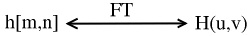
The blurring can usually be modeled as an LSI system with a given PSF h[ m, n] .
Figure 1.1.
Fourier Transform (FT) relationship between the two functions.
The observed image is
()
g[ m, n]= h[ m, n]* f[ m, n]
()
G( u, v)= H( u, v) F( u, v)
()
Example 1.1. Image Blurring
Above we showed the equations for representing the common model for blurring an image. In
Figure 1.2 we have an original image and a PSF function that we wish to apply to the image in order to model a basic blurred image.
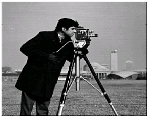

(b)
(a)
Figure 1.2.
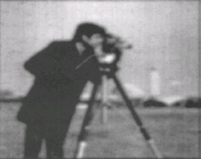
Once we apply the PSF to the original image, we receive our blurred image that is shown in
Figure 1.3.
Frequency Domain Analysis
Example 1.1 looks at the original images in its typical form; however, it is often useful to look at our images and PSF in the frequency domain. In Figure 1.4, we take another look at the image blurring example above and look at how the images and results would appear in the frequency
domain if we applied the fourier transforms.
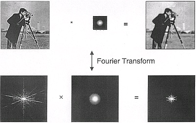
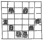

Figure 1.4.
1.2. Digital Image Processing Basics*
Digital Image Processing
A sampled image gives us our usual 2D array of pixels f[ m, n] (Figure 1.5): Figure 1.5.
We illustrate a "pixelized" smiley face.
We can filter f[ m, n] by applying a 2D discrete-space convolution as shown below (where h[ m, n] is our PSF):
()
Example 1.2. Sampled Image
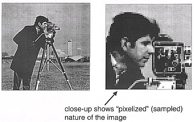

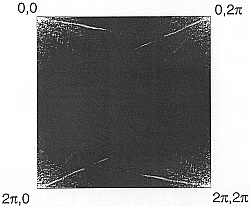
Figure 1.6.
Illustrate the "pixelized" nature of all digital images.
We also have discrete-space FTS:
()
where F[ u, v] is analogous to DTFT in 1D.
"Convolution in Time" is the same as "Multiplication in Frequency"
()
g[ m, n]= h[ m, n]* f[ m, n]
which, as stated above, is the same as:
()
G[ u, v]= H[ u, v] F[ u, v]
Example 1.3. Magnitude of FT of Cameraman Image

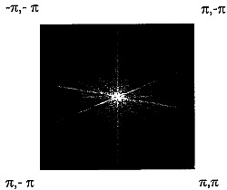


Figure 1.7.
To get a better image, we can use the fftshift command in Matlab to center the Fourier
Transform. The resulting image is shown in Figure 1.8:
Figure 1.8.
1.3. 2D DFT*
2D DFT
To perform image restoration (and many other useful image processing algorithms) in a computer,
we need a Fourier Transform (FT) that is discrete and two-dimensional.
()
for k={0, …, N−1} and l={0, …, N−1} .
()
()
where the above equation (Equation) has finite support for an N x N image.


Inverse 2D DFT
As with our regular fourier transforms, the 2D DFT also has an inverse transform that allows us to
reconstruct an image as a weighted combination of complex sinusoidal basis functions.
()
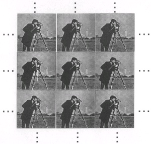
Example 1.4. Periodic Extensions
Figure 1.9.
Illustrate the periodic extension of images.
2D DFT and Convolution
The regular 2D convolution equation is
()
Example 1.5.
Below we go through the steps of convolving two two-dimensional arrays. You can think of f
as r