Intro to Digital Signal Processing by Robert Nowak, et al - HTML preview
Download the book in PDF, ePub for a complete version.


simple a matter of taking the z-transform formula, H( z) , and replacing every instance of z with ⅇⅈw .
()
Once you understand the derivation of this formula, look at the module concerning Filter Design
from the Z-Transform for a look into how all of these ideas of the Z-transform, Difference
Equation, and Pole/Zero Plots play a role in filter design.
Example
Example 3.1. Finding Difference Equation
Below is a basic example showing the opposite of the steps above: given a transfer function
one can easily calculate the systems difference equation.
()
Given this transfer function of a time-domain filter, we want to find the difference equation.
To begin with, expand both polynomials and divide them by the highest order z.
()
From this transfer function, the coefficients of the two polynomials will be our ak and
bk values found in the general difference equation formula, Equation. Using these coefficients and the above form of the transfer function, we can easily write the difference equation:
()
In our final step, we can rewrite the difference equation in its more common form showing the
recursive nature of the system.
()
Solving a LCCDE


In order for a linear constant-coefficient difference equation to be useful in analyzing a LTI
system, we must be able to find the systems output based upon a known input, x( n) , and a set of
initial conditions. Two common methods exist for solving a LCCDE: the direct method and the
indirect method, the later being based on the z-transform. Below we will briefly discuss the
formulas for solving a LCCDE using each of these methods.
Direct Method
The final solution to the output based on the direct method is the sum of two parts, expressed in
the following equation:
()
y( n)= yh( n)+ yp( n)
The first part, yh( n) , is referred to as the homogeneous solution and the second part, yh( n) , is referred to as particular solution. The following method is very similar to that used to solve
many differential equations, so if you have taken a differential calculus course or used differential
equations before then this should seem very familiar.
Homogeneous Solution
We begin by assuming that the input is zero, x( n)=0 . Now we simply need to solve the
homogeneous difference equation:
()
In order to solve this, we will make the assumption that the solution is in the form of an
exponential. We will use lambda, λ, to represent our exponential terms. We now have to solve the
following equation:
()
We can expand this equation out and factor out all of the lambda terms. This will give us a large
polynomial in parenthesis, which is referred to as the characteristic polynomial. The roots of this
polynomial will be the key to solving the homogeneous equation. If there are all distinct roots,
then the general solution to the equation will be as follows:
()
yh( n)= C 1( λ 1) n+ C 2( λ 2) n+ …+ CN( λN) n However, if the characteristic equation contains multiple roots then the above general solution
will be slightly different. Below we have the modified version for an equation where λ1 has K
multiple roots:


()
yh( n)= C 1( λ 1) n+ C 1 n( λ 1) n+ C 1 n 2( λ 1) n+ …+ C 1 nK−1( λ 1) n+ C 2( λ 2) n+ …+ CN( λN) n Particular Solution
The particular solution, yp( n) , will be any solution that will solve the general difference equation: ()
In order to solve, our guess for the solution to yp( n) will take on the form of the input, x( n) . After guessing at a solution to the above equation involving the particular solution, one only needs to
plug the solution into the difference equation and solve it out.
Indirect Method
The indirect method utilizes the relationship between the difference equation and z-transform,
discussed earlier, to find a solution. The basic idea is to convert the difference equation into a z-transform, as described above, to get the resulting output, Y( z) . Then by inverse transforming this and using partial-fraction expansion, we can arrive at the solution.
(3.1)
Z { y ( n + 1 ) – y ( n ) } = z Y ( z ) – y ( 0 ) This can be interatively extended to an arbitrary order derivative as in Equation Equation 3.2.
(3.2)
Now, the Laplace transform of each side of the differential equation can be taken
(3.3)
which by linearity results in
(3.4)
and by differentiation properties in
(3.5)
Rearranging terms to isolate the Laplace transform of the output,


(3.6)
Thus, it is found that
(3.7)
In order to find the output, it only remains to find the Laplace transform X( z) of the input,
substitute the initial conditions, and compute the inverse Z-transform of the result. Partial fraction
expansions are often required for this last step. This may sound daunting while looking at
Equation 3.7, but it is often easy in practice, especially for low order difference equations.
Equation 3.7 can also be used to determine the transfer function and frequency response.
As an example, consider the difference equation
(3.8)
y [ n - 2 ] + 4 y [ n - 1 ] + 3 y [ n ] = cos ( n ) with the initial conditions y'(0)=1 and y(0)=0 Using the method described above, the Z transform
of the solution y[ n] is given by
(3.9)
Performing a partial fraction decomposition, this also equals
(3.10)
Computing the inverse Laplace transform,
(3.11)
One can check that this satisfies that this satisfies both the differential equation and the initial
conditions.
3.2. The Z Transform: Definition*
Basic Definition of the Z-Transform
The z-transform of a sequence is defined as


()
Sometimes this equation is referred to as the bilateral z-transform. At times the z-transform is
defined as
()
which is known as the unilateral z-transform.
There is a close relationship between the z-transform and the Fourier transform of a discrete
time signal, which is defined as
()
Notice that that when the z– n is replaced with ⅇ–( ⅈωn) the z-transform reduces to the Fourier Transform. When the Fourier Transform exists, z= ⅇⅈω , which is to have the magnitude of z equal to unity.
The Complex Plane
In order to get further insight into the relationship between the Fourier Transform and the Z-
Transform it is useful to look at the complex plane or z-plane. Take a look at the complex plane:
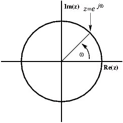
Figure 3.1. Z-Plane
The Z-plane is a complex plane with an imaginary and real axis referring to the complex-valued
variable z. The position on the complex plane is given by rⅇⅈω , and the angle from the positive, real axis around the plane is denoted by ω. X( z) is defined everywhere on this plane. X( ⅇⅈω ) on the other hand is defined only where | z|=1 , which is referred to as the unit circle. So for example,
ω=1 at z=1 and
at z=-1. This is useful because, by representing the Fourier transform as the


z-transform on the unit circle, the periodicity of Fourier transform is easily seen.
Region of Convergence
The region of convergence, known as the ROC, is important to understand because it defines the
region where the z-transform exists. The ROC for a given x[ n] , is defined as the range of z for which the z-transform converges. Since the z-transform is a power series, it converges when
x[ n] z– n is absolutely summable. Stated differently,
()
must be satisfied for convergence. This is best illustrated by looking at the different ROC's of the
z-transforms of αnu[ n] and αnu[ n−1] .
Example 3.2.
For
()
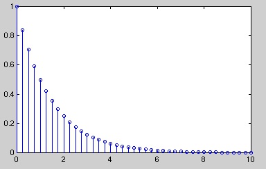
x[ n]= αnu[ n]
Figure 3.2.
x[ n]= αnu[ n] where α=0.5.
()
This sequence is an example of a right-sided exponential sequence because it is nonzero for


n≥0 . It only converges when | αz-1|<1 . When it converges,
()
If | αz-1|≥1 , then the series,
does not converge. Thus the ROC is the range of values
where
()
| αz-1|<1
or, equivalently,
()
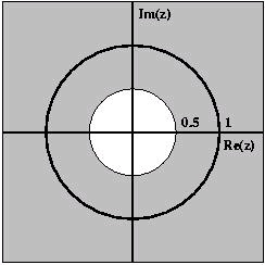
| z|>| α|
Figure 3.3.
ROC for x[ n]= αnu[ n] where α=0.5
Example 3.3.
For
()
x[ n]=(–( αn)) u[– n−1]
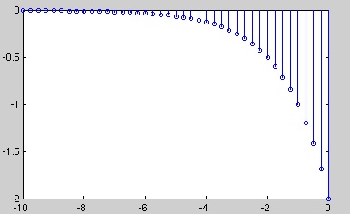


Figure 3.4.
x[ n]=(–( αn)) u[– n−1] where α=0.5.
()
The ROC in this case is the range of values where
()
| α-1 z|<1
or, equivalently,
()
| z|<| α|
If the ROC is satisfied, then
()
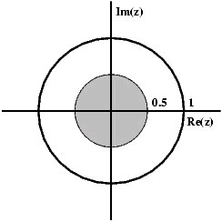


Figure 3.5.
ROC for x[ n]=(–( αn)) u[– n−1]
3.3. Table of Common z-Transforms*
The table below provides a number of unilateral and bilateral z-transforms. The table also specifies the region of convergence.
The notation for z found in the table below may differ from that found in other tables. For
example, the basic z-transform of u[ n] can be written as either of the following two
expressions, which are equivalent:
()
Table 3.1.
Signal
Z-Transform ROC
δ[ n− k]
z– k
u[ n]
| z|>1
–( u[– n−1])
| z|<1


nu[ n]
| z|>1
n 2 u[ n]
| z|>1
n 3 u[ n]
| z|>1
(–( αn)) u[– n−1]
| z|<|α|
αnu[ n]
| z|>| α|
nαnu[ n]
| z|>| α|
n 2 αnu[ n]
| z|>| α|
γn cos( αn) u[ n]
| z|>| γ|
γn sin( αn) u[ n]
| z|>| γ|
3.4. Poles and Zeros*
Introduction
It is quite difficult to qualitatively analyze the Laplace transform and Z-transform, since mappings of their magnitude and phase or real part and imaginary part result in multiple
mappings of 2-dimensional surfaces in 3-dimensional space. For this reason, it is very common to
examine a plot of a transfer function's poles and zeros to try to gain a qualitative idea of what a system does.
Given a continuous-time transfer function in the Laplace domain, H( s) , or a discrete-time one in
the Z-domain, H( z) , a zero is any value of s or z such that the transfer function is zero, and a pole is any value of s or z such that the transfer function is infinite. To define them precisely:
Definition: zeros
1. The value(s) for z where the numerator of the transfer function equals zero


2. The complex frequencies that make the overall gain of the filter transfer function zero.
Definition: poles
1. The value(s) for z where the denominator of the transfer function equals zero
2. The complex frequencies that make the overall gain of the filter transfer function infinite.
Pole/Zero Plots
When we plot these in the appropriate s- or z-plane, we represent zeros with "o" and poles with
"x". Refer to this module for a detailed looking at plotting the poles and zeros of a z-transform on the Z-plane.
Example 3.4.
Find the poles and zeros for the transfer function
and plot the results in the s-
plane.
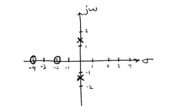
The first thing we recognize is that this transfer function will equal zero whenever the top,
s 2+6 s+8 , equals zero. To find where this equals zero, we factor this to get, ( s+2)( s+4) . This yields zeros at s=-2 and s=-4 . Had this function been more complicated, it might have been
necessary to use the quadratic formula.
For poles, we must recognize that the transfer function will be infinite whenever the bottom
part is zero. That is when s 2+2 is zero. To find this, we again look to factor the equation. This
yields
. This yields purely imaginary roots of
and
Plotting this gives Figure 3.6
Figure 3.6. Pole and Zero Plot
Sample pole-zero plot


Now that we have found and plotted the poles and zeros, we must ask what it is that this plot gives
us. Basically what we can gather from this is that the magnitude of the transfer function will be
larger when it is closer to the poles and smaller when it is closer to the zeros. This provides us
with a qualitative understanding of what the system does at various frequencies and is crucial to
the discussion of stability.
Repeated Poles and Zeros
It is possible to have more than one pole or zero at any given point. For instance, the discrete-time
transfer function H( z)= z 2 will have two zeros at the origin and the continuous-time function will have 25 poles at the origin.
Pole-Zero Cancellation
An easy mistake to make with regards to poles and zeros is to think that a function like
is the same as s+3 . In theory they are equivalent, as the pole and zero at s=1 cancel each other
out in what is known as pole-zero cancellation. However, think about what may happen if this
were a transfer function of a system that was created with physical circuits. In this case, it is very
unlikely that the pole and zero would remain in exactly the same place. A minor temperature
change, for instance, could cause one of them to mov