LabVIEW Graphical Programming by Serhat Beyenir - HTML preview
Download the book in PDF, ePub, Kindle for a complete version.
Chapter 3
Repetition and Loops
3.1 While Loops1
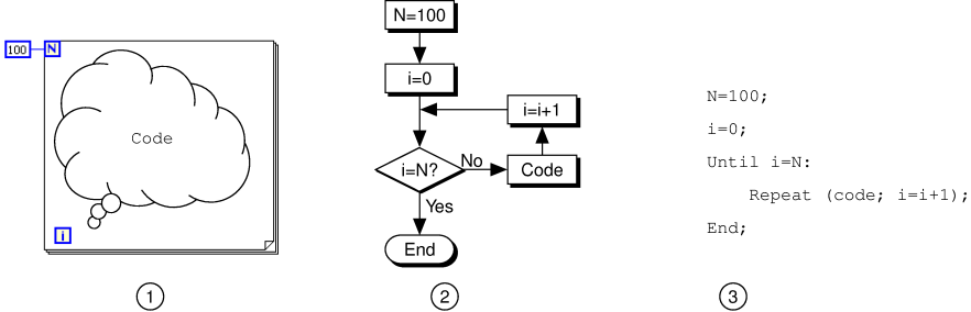
A ❲❤✐❧❡ ▲♦♦♣ executes a subdiagram until a condition is met. The ❲❤✐❧❡ ▲♦♦♣ is similar to a ❉♦ ▲♦♦♣ or a
❘❡♣❡❛t✲❯♥t✐❧ ▲♦♦♣ in text-based programming. Figure 3.1 shows a ❲❤✐❧❡ ▲♦♦♣ in LabVIEW, a flow chart
equivalent of the ❲❤✐❧❡ ▲♦♦♣ functionality, and a pseudo code example of the functionality of the ❲❤✐❧❡
▲♦♦♣.
Figure 3.1
The ❲❤✐❧❡ ▲♦♦♣ is located on the ❋✉♥❝t✐♦♥s
❊①❡❝✉t✐♦♥ ❈♦♥tr♦❧ palette. Select the ❲❤✐❧❡ ▲♦♦♣ from
the palette then use the cursor to drag a selection rectangle around the section of the block diagram you want to repeat. When you release the mouse button, a ❲❤✐❧❡ ▲♦♦♣ boundary encloses the section you
selected.
Add block diagram objects to the ❲❤✐❧❡ ▲♦♦♣ by dragging and dropping them inside the ❲❤✐❧❡ ▲♦♦♣.
NOTE: The ❲❤✐❧❡ ▲♦♦♣ always executes at least once.
The ❲❤✐❧❡ ▲♦♦♣ executes the subdiagram until the conditional terminal, an input terminal, receives
a specific Boolean value. The default behavior and appearance of the conditional terminal is ❙t♦♣ ■❢ ❚r✉❡, shown in this media. When a conditional terminal is ❙t♦♣ ■❢ ❚r✉❡, the ❲❤✐❧❡ ▲♦♦♣ executes its subdiagram until the conditional terminal receives a ❚r✉❡ value.
The ✐t❡r❛t✐♦♥ terminal, an output terminal, shown in this media, contains the number of com-
pleted iterations. The iteration count always starts at zero. During the first iteration, the iteration terminal returns ✵.
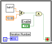
In the block diagram in Figure 3.2, the ❲❤✐❧❡ ▲♦♦♣ executes until the subVI output is greater than or equal to ✶✵✳✵✵ and the ❊♥❛❜❧❡ control is ❚r✉❡. The ❆♥❞ function returns ❚r✉❡ only if both inputs are ❚r✉❡.
Otherwise, it returns ❋❛❧s❡.
1This content is available online at <http://cnx.org/content/m12212/1.2/>.
Available for free at Connexions <http://cnx.org/content/col11408/1.1>
67

68
CHAPTER 3. REPETITION AND LOOPS
Figure 3.2
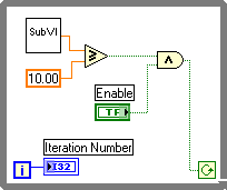
In the previous example (Figure 3.2), there is an increased probability of an infinite loop. Generally, the desired behavior is to have one condition met to stop the loop, rather than requiring both conditions to be met.
You can change the behavior and appearance of the conditional terminal by right-clicking the ter-
minal or the border of the ❲❤✐❧❡ ▲♦♦♣ and selecting ❈♦♥t✐♥✉❡ ✐❢ ❚r✉❡, shown at left. You also can use the
❖♣❡r❛t✐♥❣ tool to click the conditional terminal to change the condition. When a conditional terminal is
❈♦♥t✐♥✉❡ ✐❢ ❚r✉❡, the ❲❤✐❧❡ ▲♦♦♣ executes its subdiagram until the conditional terminal receives a ❋❛❧s❡
value, as shown in Figure 3.3.
Figure 3.3
The ❲❤✐❧❡ ▲♦♦♣ executes until the subVI output is less than ✶✵✳✵✵ or the ❊♥❛❜❧❡ control is ❋❛❧s❡.
3.1.1 Structure Tunnels
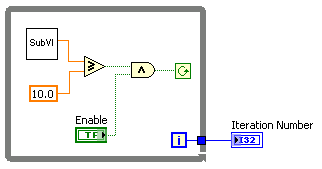
Data can be passed out of or into a ❲❤✐❧❡ ▲♦♦♣ through a tunnel. Tunnels feed data into and out of structures. The tunnel appears as a solid block on the border of the ❲❤✐❧❡ ▲♦♦♣. The block is the color of the data type wired to the tunnel. Data pass out of a loop after the loop terminates. When a tunnel passes data into a loop, the loop executes only after data arrive at the tunnel.
In Figure 3.4, the ✐t❡r❛t✐♦♥ terminal is connected to a tunnel. The value in the tunnel does not get passed to the ■t❡r❛t✐♦♥ ◆✉♠❜❡r indicator until the ❲❤✐❧❡ ▲♦♦♣ has finished execution.
Available for free at Connexions <http://cnx.org/content/col11408/1.1>


69
Figure 3.4
Only the last value of the iteration terminal displays in the ■t❡r❛t✐♦♥ ◆✉♠❜❡r indicator.
3.2 For Loops2
A ❋♦r ▲♦♦♣ executes a subdiagram a set number of times. Figure 3.5 shows a ❋♦r ▲♦♦♣ in LabVIEW, a flow chart equivalent of the ❋♦r ▲♦♦♣ functionality, and a pseudo code example of the functionality of the ❋♦r
▲♦♦♣.
Figure 3.5
The ❋♦r ▲♦♦♣ is located on the ❋✉♥❝t✐♦♥s
❆❧❧ ❋✉♥❝t✐♦♥s ❙tr✉❝t✉r❡s palette. You also can
place a ❲❤✐❧❡ ▲♦♦♣ on the block diagram, right-click the border of the ❲❤✐❧❡ ▲♦♦♣, and select ❘❡♣❧❛❝❡
✇✐t❤ ❋♦r ▲♦♦♣ from the shortcut menu to change a ❲❤✐❧❡ ▲♦♦♣ to a ❋♦r ▲♦♦♣. The value in the ❝♦✉♥t
terminal (an input terminal), shown in this media, indicates how many times to repeat the subdiagram.
The ✐t❡r❛t✐♦♥ terminal (an output terminal), shown in this media, contains the number of com-
pleted iterations. The iteration count always starts at zero. During the first iteration, the iteration terminal returns ✵.
The ❋♦r ▲♦♦♣ differs from the ❲❤✐❧❡ ▲♦♦♣ in that the ❋♦r ▲♦♦♣ executes a set number of times. A ❲❤✐❧❡
▲♦♦♣ stops executing the subdiagram only if the value at the conditional terminal exists.
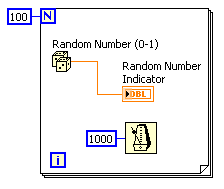
The ❋♦r ▲♦♦♣ in Figure 3.6 generates a random number every second for 100 seconds and displays the
random numbers in a numeric indicator.
2This content is available online at <http://cnx.org/content/m12214/1.2/>.
Available for free at Connexions <http://cnx.org/content/col11408/1.1>


70
CHAPTER 3. REPETITION AND LOOPS
Figure 3.6
3.2.1 Wait Functions
The ❲❛✐t ❯♥t✐❧ ◆❡①t ♠s ▼✉❧t✐♣❧❡ function, shown in this media, monitors a millisecond counter
and waits until the millisecond counter reaches a multiple of the amount you specify. Use this function to synchronize activities. Place this function within a loop to control the loop execution rate.
The ❲❛✐t ✭♠s✮ function, shown in this media, adds the wait time to the code execution time. This
can cause a problem if code execution time is variable.
NOTE: The ❚✐♠❡ ❉❡❧❛② Express VI, located on the ❋✉♥❝t✐♦♥s
❊①❡❝✉t✐♦♥ ❈♦♥tr♦❧ palette, be-
haves similar to the ❲❛✐t ✭♠s✮ function with the addition of built-in error clusters. Refer to Clus-
ters3 for more information about error clusters.
3.2.2 Wait Functions
LabVIEW can represent numeric data types as signed or unsigned integers (8-bit, 16-bit, or 32-bit), floating-point numeric values (single-, double-, or extended-precision), or complex numeric values (single-, double-
, or extended-precision). When you wire two or more numeric inputs of different representations to a function, the function usually returns output in the larger or wider format. The functions coerce the smaller representations to the widest representation before execution, and LabVIEW places a coercion dot on the terminal where the conversion takes place.
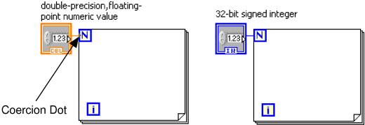
For example, the ❋♦r ▲♦♦♣ count terminal is a 32-bit signed integer. If you wire a double-precision, floating-point numeric to the count terminal, LabVIEW converts the numeric to a 32-bit signed integer. A coercion dot appears on the count terminal of the first ❋♦r ▲♦♦♣, as shown in Figure 3.7.
Figure 3.7
3"Error Clusters" <http://cnx.org/content/m12231/latest/>
Available for free at Connexions <http://cnx.org/content/col11408/1.1>
71
If you wire two different numeric data types to a numeric function that expects the inputs to be the same data type, LabVIEW converts one of the terminals to the same representation as the other terminal.
LabVIEW chooses the representation that uses more bits. If the number of bits is the same, LabVIEW
chooses unsigned over signed.
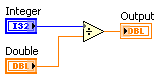
In the example in Figure 3.8, a 32-bit signed integer (I32) and a double-precision, floating-point numeric value (DBL) are wired to the ❉✐✈✐❞❡ function. The 32-bit signed integer is coerced since it uses fewer bits than the double-precision, floating-point numeric value.
Figure 3.8
To change the representation of a numeric object, right-click the object and select ❘❡♣r❡s❡♥t❛t✐♦♥ from the shortcut menu. Select the data type that best represents the ❞❛t❛✳✉t data types.
When LabVIEW converts double-precision, floating-point numeric values to integers, it rounds to the
nearest integer. LabVIEW rounds ①✳✺ to the nearest even integer. For example, LabVIEW rounds 2.5 to 2
and 3.5 to 4.
Refer to the Data Types section of Introduction to LabVIEW, of this manual or to the LabVIEW Help for more information about data types.
3.3 Timed Temperature VI4
Exercise 3.3.1
Complete the following steps to build a VI that uses the Thermometer VI to read a temperature
once every second for a duration of one minute.
3.3.1 Front Panel
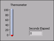
1. Open a blank VI and build the front panel shown in Figure 3.9.
Figure 3.9
4This content is available online at <http://cnx.org/content/m12216/1.1/>.
Available for free at Connexions <http://cnx.org/content/col11408/1.1>


72
CHAPTER 3. REPETITION AND LOOPS
a. Place a t❤❡r♠♦♠❡t❡r, located on the ❈♦♥tr♦❧s
◆✉♠❡r✐❝ ■♥❞✐❝❛t♦rs palette, on the
front panel. This provides a visual indication of the temperature reading.
b. Place a ♥✉♠❡r✐❝ ✐♥❞✐❝❛t♦r, located on the ❈♦♥tr♦❧s
◆✉♠❡r✐❝ ■♥❞✐❝❛t♦rs palette,
on the front panel. Label this indicator ❙❡❝♦♥❞s ❊❧❛♣s❡❞. Right-click the indicator and
select ❘❡♣r❡s❡♥t❛t✐♦♥
■✸✷ from the shortcut menu.
3.3.2 Block Diagram
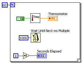
1. Build the block diagram shown in Figure 3.10.
Figure 3.10
-
Place a ❋♦r ▲♦♦♣, located on the ❋✉♥❝t✐♦♥s
❆❧❧ ❋✉♥❝t✐♦♥s ❙tr✉❝t✉r❡s
palette, on the block diagram. Right-click the ▲♦♦♣ ❈♦✉♥t terminal in the upper
left corner of the ❋♦r ▲♦♦♣ and select ❈r❡❛t❡ ❈♦♥st❛♥t from the shortcut menu.
Type ✻✵ in the constant to set the ❋♦r ▲♦♦♣ to repeat 60 times.
-
Place the ❚❤❡r♠♦♠❡t❡r VI on the block diagram. Select ❋✉♥❝t✐♦♥s
❆❧❧
❋✉♥❝t✐♦♥s ❙❡❧❡❝t ❛ ❱■ and navigate to ❈✿\❊①❡r❝✐s❡s\▲❛❜❱■❊❲ ❇❛s✐❝s
■\❚❤❡r♠♦♠❡t❡r✳✈✐to place the VI. This VI reads the temperature from the DAQ
device. Right-click the ❚❡♠♣ ❙❝❛❧❡ input and select ❈r❡❛t❡
❈♦♥st❛♥t from
the shortcut menu. Use a ❋❛❧s❡ constant for Fahrenheit or a ❚r✉❡ constant for
Celsius.
NOTE: If you do not have a DAQ device with a temperature sensor on Channel 0, use
the ✭❉❡♠♦✮ ❚❤❡r♠♦♠❡t❡r VI instead.
-
Place the ❲❛✐t ❯♥t✐❧ ◆❡①t ♠s ▼✉❧t✐♣❧❡ function,
located on the
❋✉♥❝t✐♦♥s ❆❧❧ ❋✉♥❝t✐♦♥s ❚✐♠❡ ✫ ❉✐❛❧♦❣ palette, on the block diagram.
Right-click the input and select ❈r❡❛t❡
❈♦♥st❛♥t from the shortcut menu. Enter
a value of ✶✵✵✵ to set the wait to every second.
-
Place the ■♥❝r❡♠❡♥t function, located on the ❋✉♥❝t✐♦♥s
❆r✐t❤♠❡t✐❝ ✫
❈♦♠♣❛r✐s♦♥ ❊①♣r❡ss ◆✉♠❡r✐❝ palette, on the block diagram. This function
adds one to the iteration terminal output.
Available for free at Connexions <http://cnx.org/content/col11408/1.1>
73
2. Save this VI as ❚✐♠❡❞ ❚❡♠♣❡r❛t✉r❡✳✈✐ in the ❈✿\❊①❡r❝✐s❡s\▲❛❜❱■❊❲ ❇❛s✐❝s ■ directory.
3. Run the VI. The first reading might take longer than one second to retrieve if the computer
needs to configure the DAQ device.
4. If time permits, complete the following optional and challenge steps, otherwise close the VI.
3.3.3 Optional
1. Build a VI that generates random numbers in a ❲❤✐❧❡ ▲♦♦♣ and stops when you click a stop
button on the front panel.
2. Save the VI as ●❡♥❡r❛❧ ❲❤✐❧❡ ▲♦♦♣✳✈✐ in the ❈✿\❊①❡r❝✐s❡s\▲❛❜❱■❊❲ ❇❛s✐❝s ■ directory.
3.3.4 Challenge
1. Modify the ●❡♥❡r❛❧ ❲❤✐❧❡ ▲♦♦♣ VI to stop when the stop button is clicked or when the
❲❤✐❧❡ ▲♦♦♣ reaches a number of iterations specified by a front panel control.
2. Select
❋✐❧❡ ❙❛✈❡ ❆s to save the VI as ❈♦♠❜♦ ❲❤✐❧❡✲❋♦r ▲♦♦♣✳✈✐ in the
❈✿\❊①❡r❝✐s❡s\▲❛❜❱■❊❲ ❇❛s✐❝s ■ directory.
Available for free at Connexions <http://cnx.org/content/col11408/1.1>
74
CHAPTER 3. REPETITION AND LOOPS
3.4 Summary, Tips, and Tricks on Repetition and Loops5
• Use structures on the block diagram to repeat blocks of code and to execute code conditionally or in a specific order.
• The ❲❤✐❧❡ ▲♦♦♣ executes the subdiagram until the ❝♦♥❞✐t✐♦♥❛❧ terminal receives a specific Boolean
value. By default, the ❲❤✐❧❡ ▲♦♦♣ executes its subdiagram until the conditional terminal receives a
❚r✉❡ value.
• The ❋♦r ▲♦♦♣ executes a subdiagram a set number of times.
• You create loops by using the cursor to drag a selection rectangle around the section of the block diagram you want to repeat or by dragging and dropping block diagram objects inside the loop.
• The ❲❛✐t ❯♥t✐❧ ◆❡①t ♠s ▼✉❧t✐♣❧❡ function makes sure that each iteration occurs at certain inter-
vals. Use this function to add timing to loops.
• The ❲❛✐t ✭♠s✮ function waits a set amount of time.
• Coercion dots appear where LabVIEW coerces a numeric representation of one terminal to match the
numeric representation of another terminal.
• Use s❤✐❢t r❡❣✐st❡rs on ❋♦r ▲♦♦♣s and ❲❤✐❧❡ ▲♦♦♣s to transfer values from one loop iteration to
the next.
• Create a s❤✐❢t r❡❣✐st❡r by right-clicking the left or right border of a loop and selecting ❆❞❞ ❙❤✐❢t
❘❡❣✐st❡r from the shortcut menu.
• To configure a s❤✐❢t r❡❣✐st❡r to carry over values to the next iteration, right-click the left terminal and select ❆❞❞ ❊❧❡♠❡♥t from the shortcut menu.
• The ❋❡❡❞❜❛❝❦ ◆♦❞❡ stores data when the loop completes an iteration, sends that value to the next
iteration of the loop, and transfers any data type.
• Use the ❋❡❡❞❜❛❝❦ ◆♦❞❡ to avoid unnecessarily long wires.
5This content is available online at <http://cnx.org/content/m12219/1.1/>.
Available for free at Connexions <http://cnx.org/content/col11408/1.1>