ECE 320 Spring 2004 by Mark Butala, et al - HTML preview
Download the book in PDF, ePub for a complete version.
17
18 // Initial PN generator register contents
19 int seed = 1;
20
21 // Initial phase
22 int prev_phase = 0;
23
24
25 while( 1 )
26 {
27 /* Wait for a new block of samples */
28 WaitAudio(&Rcvptr,&Xmitptr);
29
30 // Get next two random bits
31 r1 = randbit( &seed );
32 r2 = randbit( &seed );
33 // Convert 2 bit binary number to decimal
34 symbol = series2parallel(r1,r2);
35
36 for (n=0; n<32; n++)
37 {
38 phase[n] = ( freqs[symbol]*n + prev_phase ) % 64; // get into 0 to 64 range
39 if (phase[n] > 32) phase[n]=phase[n]-64; // get into -32 to 32 range
40 phase[n] = phase[n] * 1024; // 1024=2^15*1/32
41 // [-2^15 2^15] range for use with
42 // SINE.asm
43 }
44 sine(&phase[0], &output[0], 32); // compute SINE, put result in output[0 -
31]
45 prev_phase = ( freqs[symbol]*32 + prev_phase ) % 64; // save current phase offset
46
47 // Get next two random bits
48 r1 = randbit( &seed );
49 r2 = randbit( &seed );
50 // Convert 2 bit binary number to decimal
51 symbol = series2parallel(r1,r2);
52
53 for (n=0; n<32; n++)
54 {
55 phase[n] = ( freqs[symbol]*n + prev_phase ) % 64;
56 if (phase[n] > 32) phase[n]=phase[n]-64;
57 phase[n] = phase[n] * 1024;
58 }
59 sine(&phase[0], &output[32], 32);
60 prev_phase = ( freqs[symbol]*32 + prev_phase ) % 64;
61
62
63 // Transfer the two symbols to transmit buffer
64 for (n=0; n<64; n++)
65 {
66 Xmitptr[6*n] = output[n];
67 }
68
69 }
70 }
71
72
73 // Converts 2 bit binary number (r2r1) to decimal
74 int series2parallel(int r2, int r1)
75 {
76 if ((r2==0)&&(r1==0)) return 0;
77 else if ((r2==0)&&(r1==1)) return 1;
78 else if ((r2==1)&&(r1==0)) return 2;
79 else return 3;
80 }
81
82 //Returns as an integer a random bit, based on the 15 low-significance bits in iseed (which is
83 //modified for the next call).
84 int randbit(unsigned int *iseed)
85 {
86 unsigned int newbit; // The accumulated XORs.
87 newbit = (*iseed >> 14) & 1 ^ (*iseed >> 13) & 1; // XOR bit 15 and bit 14
88 // Leftshift the seed and put the result of the XORs in its bit 1.
89 *iseed=(*iseed << 1) | newbit;
90 return (int) newbit;
91 }
Solutions

Chapter 2. Project Labs
2.1. Adaptive Filtering
Adaptive Filtering: LMS Algorithm*
Introduction
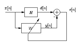
Figure 2.1 is a block diagram of system identification using adaptive filtering. The objective is to change (adapt) the coefficients of an FIR filter, W , to match as closely as possible the response of
an unknown system, H . The unknown system and the adapting filter process the same input signal
x[ n] and have outputs d[ n] (also referred to as the desired signal) and y[ n] .
Figure 2.1.
System identification block diagram.
Gradient-descent adaptation
The adaptive filter, W , is adapted using the least mean-square algorithm, which is the most
widely used adaptive filtering algorithm. First the error signal, e[ n] , is computed as
e[ n]= d[ n]− y[ n] , which measures the difference between the output of the adaptive filter and the output of the unknown system. On the basis of this measure, the adaptive filter will change its
coefficients in an attempt to reduce the error. The coefficient update relation is a function of the
error signal squared and is given by
()
The term inside the parentheses represents the gradient of the squared-error with respect to the
i th coefficient. The gradient is a vector pointing in the direction of the change in filter coefficients


that will cause the greatest increase in the error signal. Because the goal is to minimize the error,
however, Equation updates the filter coefficients in the direction opposite the gradient; that is why the gradient term is negated. The constant μ is a step-size, which controls the amount of gradient
information used to update each coefficient. After repeatedly adjusting each coefficient in the
direction opposite to the gradient of the error, the adaptive filter should converge; that is, the
difference between the unknown and adaptive systems should get smaller and smaller.
To express the gradient decent coefficient update equation in a more usable manner, we can
rewrite the derivative of the squared-error term as
()
()
which in turn gives us the final LMS coefficient update,
()
h n+1[ i]= hn[ i]+ μex[ n− i]
The step-size μ directly affects how quickly the adaptive filter will converge toward the unknown
system. If μ is very small, then the coefficients change only a small amount at each update, and
the filter converges slowly. With a larger step-size, more gradient information is included in each
update, and the filter converges more quickly; however, when the step-size is too large, the
coefficients may change too quickly and the filter will diverge. (It is possible in some cases to
determine analytically the largest value of μ ensuring convergence.)
MATLAB Simulation
Simulate the system identification block diagram shown in Figure 2.1.
Previously in MATLAB, you used the filter command or the conv command to implement
shift-invariant filters. Those commands will not work here because adaptive filters are shift-
varying, since the coefficient update equation changes the filter's impulse response at every
sample time. Therefore, implement the system identification block on a sample-by-sample basis
with a do loop, similar to the way you might implement a time-domain FIR filter on a DSP. For
the "unknown" system, use the fourth-order, low-pass, elliptical, IIR filter designed for the IIR
Filtering: Filter-Design Exercise in MATLAB.
Use Gaussian random noise as your input, which can be generated in MATLAB using the
command randn. Random white noise provides signal at all digital frequencies to train the
adaptive filter. Simulate the system with an adaptive filter of length 32 and a step-size of 0.02 .
Initialize all of the adaptive filter coefficients to zero. From your simulation, plot the error (or
squared-error) as it evolves over time and plot the frequency response of the adaptive filter
coefficients at the end of the simulation. How well does your adaptive filter match the "unknown"
filter? How long does it take to converge?
Once your simulation is working, experiment with different step-sizes and adaptive filter lengths.
Processor Implementation
Use the same "unknown" filter as you used in the MATLAB simulation.
Although the coefficient update equation is relatively straightforward, consider using the lms
instruction available on the TI processor, which is designed for this application and yields a very
efficient implementation of the coefficient update equation.
To generate noise on the DSP, you can use the PN generator from the Digital Transmitter:
Introduction to Quadrature Phase-Shift Keying, but shift the PN register contents up to make the sign bit random. (If the sign bit is always zero, then the noise will not be zero-mean and this
will affect convergence.) Send the desired signal, d[ n] , the output of the adaptive filter, y[ n] , and the error to the D/A for display on the oscilloscope.
When using the step-size suggested in the MATLAB simulation section, you should notice that the
error converges very quickly. Try an extremely small μ so that you can actually watch the
amplitude of the error signal decrease towards zero.
Extensions
If your project requires some modifications to the implementation here, refer to Haykin [link] and consider some of the following questions regarding such modifications:
How would the system in Figure 2.1 change for different applications? (noise cancellation,
equalization, etc. )
What happens to the error when the step-size is too large or too small?
How does the length of an adaptive FIR filters affect convergence?
What types of coefficient update relations are possible besides the described LMS algorithm?
References
1. S. Haykin. (1996). Adaptive Filter Theory. (3rd edition). Prentice Hall.
2.2. Audio Effects
Audio Effects: Real-Time Control with the Serial Port*
Implementation
For this exercise, you will extend the system from Audio Effects: Using External Memory to generate a feedback-echo effect. You will then extend this echo effect to use the serial port on the
DSP EVM. The serial interface will receive data from a MATLAB GUI that allows the two system
gains and the echo delay to be changed using on-screen sliders.
Feedback system implementation
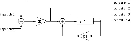
Figure 2.2.
Feedback System with Test Points
First, modify code from Audio Effects: Using External Memory to create the feedback-echo system shown in Figure 2.2. A one-tap feedback-echo is a simple audio effect that sounds
remarkably good. You will use both channels of input by summing the two inputs so that either or
both may be used as an input to the system. Also, send several test signals to the six-channel
board's D/A converters:
The summed input signal
The input signal after gain stage G 1
The data going into the long delay
The data coming out of the delay
You will also need to set both the input gain G 0 and the feedback gain G 1 to prevent overflow.
As you implement this code, ensure that the delay n and the gain values G 1 and G 2 are stored in
memory and can be easily changed using the debugger. If you do this, it will be easier to extend
your code to accept its parameters from MATLAB in MATLAB Interface Implementation.
To test your echo, connect a CD player or microphone to the input of the DSP EVM, and connect
the output of the DSP EVM to a loudspeaker. Verify that an input signal echoes multiple times in
the output and that the spacing between echoes matches the delay length you have chosen.
MATLAB interface implementation
After studying the MATLAB interface outlined at the end of Using the Serial Port with a
MATLAB GUI, write MATLAB code to send commands to the serial interface based on three sliders: two gain sliders (for G 1 and G 2 ) and one delay slider (for n). Then modify your code to
accept those commands and change the values for G 1 , G 2 and n. Make sure that n can be set to
values spanning the full range of 0 to 131,072, although it is not necessary that every number in
that range be represented.
Audio Effects: Using External Memory*
Introduction
Many audio effects require storing thousands of samples in memory on the DSP. Because there is
not enough memory on the DSP microprocessor itself to store so many samples, external memory
must be used.
In this exercise, you will use external memory to implement a long audio delay and an audio echo.
Refer to Core File: Accessing External Memory on TI TMS320C54x for a description and examples of accessing external memory.
Delay and Echo Implementation
You will implement three audio effects: a long, fixed-length delay, a variable-length delay, and a
feedback-echo.
Fixed-length delay implementation
First, implement the 131,072-sample delay shown in Figure 2.3 using the READPROG and
WRITPROG macros. Use memory locations 010000h-02ffffh in external Program RAM to do
this; you may also want to use the dld and dst opcodes to store and retrieve the 32-bit addresses
for the accumulators. Note that these two operations store the words in memory in big-endian
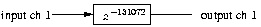
order, with the high-order word first.
Figure 2.3.
Fixed-Length Delay
Remember that arithmetic operations that act on the accumulators, such as the add instruction,
operate on the complete 32- or 40-bit value. Also keep in mind that since 131,072 is a power of
two, you can use masking (via the and instruction) to implement the circular buffer easily. This
delay will be easy to verify on the oscilloscope. (How long, in seconds, do you expect this delay to
be?)
Variable-delay implementation
Once you have your fixed-length delay working, make a copy and modify it so that the delay can
be changed to any length between zero (or one) and 131,072 samples by changing the value stored
in one double-word pair in memory. You should keep the buffer length equal to 131,072 and
change only your addressing of the sample being read back; it is more difficult to change the
buffer size to a length that is not a power of two.
Verify that your code works as expected by timing the delay from input to output and ensuring
that it is approximately the correct length.
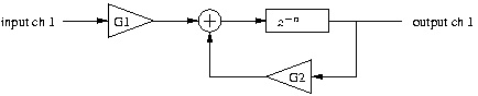
Feedback-echo implementation
Last, copy and modify your code so that the value taken from the end of the variable delay from
Variable-delay implementation is multiplied by a gain factor and then added back into the input, and the result is both saved into the delay line and sent out to the digital-to-analog converters.
Figure 2.4 shows the block diagram. (It may be necessary to multiply the input by a gain as well to prevent overflow.) This will make a one-tap feedback echo, an simple audio effect that sounds
remarkably good. To test the effect, connect the DSP EVM input to a CD player or microphone
and connect the output to a loudspeaker. Verify that the echo can be heard multiple times, and that
the spacing between echoes matches the delay length you have chosen.
Figure 2.4.
Feedback Echo
2.3. Communications
Communications: Using Direct Digital Synthesis*
Introduction
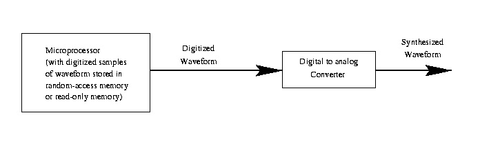
Direct Digital Synthesis ( DDS) is a method for generating a desired waveform (such as a sine
wave) by using the technique described in Figure 2.5 below.
Figure 2.5.
Direct digital synthesis (DDS) ( Couch [link])
Quantized samples of a desired waveform are stored in the memory of the microprocessor system.
This desired waveform can then be generated by "playing out" the stored words into the digital-to-
analog converter. The frequency of this waveform is determined simply by how fast the stored
words are read from memory, and is thus programmable. Likewise, the phase and amplitude of the
generated waveform are programmable.
The DDS technique is replacing analog circuits in many applications. For example, it is used in
higher-priced communication receivers to generate local oscillator signals. It can also be used to
generate sounds in electronic pipe organs and music synthesizers. Another application is its use by
lab instrument manufacturers to generate output waveforms in function generators and arbitrary
waveform generators ( Couch [link]).
In this lab you will familiarize yourself with the capabilities of the Analog Devices AD9854 DDS.
The DDS board is installed between the 6-channel card and the DSP card at some (not all) lab
stations. You can tell which boxes have them by the way the 6-channel card sits higher inside the
metal box.
Frequency Modulation (FM) Radio Exercise

To get your feet wet and see a demonstration of the DDS, perform the following exercise. Copy
the files FM.asm (downloadable here) and mod.asm from the v:\ece320\54x\dds\
directory. Assemble and run the frequency modulation (FM) program FM.asm. Next, plug an
audio source into one of the two DSP input channels that you've been using all semester. If you
have a CD on you, pop it into the computer and use that. If not, use a music web site on the
Internet as your audio source. Connect the computer to the DSP by using a male-male audio cable
and an audio-to-BNC converter box (little blue box), both of which are in the lab. The computer
has three audio outputs on the back; use the middle jack. Ask your TA if you can't find the cable
and/or box or don't see how to make the connection. Next, connect a dipole antenna to the output
of the DDS (port \#1 on the back of the DDS board). A crude but effective dipole antenna can be
formed by connecting together a few BNC and banana cables in the shape of a T. There should be
one or two of these concoctions in the lab. Once the connections are made, turn on the black
receiver in the lab, and tune it to 104.9 MHz (wide band FM). You should be able to hear your
audio source!
If your audio sounds distorted, it's most likely due to the volume of your audio source being
too loud and getting clipped by the DSP analog-to-digital converter.
Spectral Copies
Spectral Copies: The digital-to-analog converter on the DDS is unfiltered, which means that there
is no anti-imaging filter to remove the spectral replicas. To see this, plug the output of the DDS
board directly into the vector signal analyzer (VSA), and observe the spectrum. Use 104.9 MHz as
the center frequency, and set the span wide enough so that you can see the spectra of the replicas
to the left and right of the 104.9 MHz signal. Use the marker to find the peaks of the other
replicas, and record their frequencies. Once you've done that, reattach the antenna to the DDS
output, and tune the receiver to the frequencies you just recorded. You should be able to hear your
audio on each of the other frequencies.
Note
The clock rate of the DDS is 60MHz, which corresponds to 2 π in digital frequency.
Therefore, the 104.9 MHz signal you just listened to is roughly equivalent to
in digital
frequency. What are the digital frequencies of the other copies you saw on the VSA?
How to use the DDS

The DDS has several different modes of operation: single-tone, unramped Frequency Shift
Keying ( FSK), ramped FSK, chirp, and Binary Phase Shift Keying ( BPSK). In this lab we will
use the DDS in single-tone mode. Single-tone mode is easy to use, and is powerful enough to
create many different kinds of waveforms, including FM and FSK.
FM code
The FM code you just ran (also listed here) is fairly straightforward. The program first calls the
radioinit subroutine. This routine sets the DDS to single-tone mode and turns off an inverse-
sinc filter to conserve power. Following radioinit, the setcarrier subroutine is called.
This routine sets the frequency of the DDS output by writing to the two most significant 8-bit
frequency registers of the 48-bit frequency-tuning word on the DDS[3]. Although the frequency-
tuning word on the DDS has 48 bits of resolution, the upper 16 bits provide us with enough
resolution for the purposes of this lab, and so we will only be writing to the two most significant
registers. See page 26 in the DDS data sheet for a layout of the frequency-tuning word.
To set the carrier frequency, we first need to determine what frequency word has to be written to
the frequency registers on the DDS. This can be done using Equation:
()
where baseband frequency corresponds to the desired frequency that lies in the range of 0-30
MHz. For example, to get the DDS to transmit at 104.9 MHz, you would choose the baseband
frequency to be 15.1 MHz since 104.9 MHz is one of the unfiltered spectral replicas of 15.1 MHz.
Then, using Equation, the frequency word for 15.1 MHz (and 104.9 MHz) would be equal to 406D
3A06 D3D4h. But since we only write to the two most significant registers of the frequency-
tuning word, we only need the first 4 hexadecimal numbers of this result, i.e. 406Dh. The first
two of those, 40h, need to get written to the most significant 8-bit frequency register, while the
second two hex numbers, 6Dh, need to get written to the second-most significant 8-bit frequency
register. This is where the 40h and 6Dh in the setcarrier subroutine of the FM code come
from.
Writing to the frequency registers is accomplished using the portw instruction. To write to the
frequency or phase registers on the DDS, the second operand of the portw instruction must be
10xxxxxx, where the lower six bits are the address of the specific register to be written to. The
address of the most significant frequency register on the DDS is 04h, and the address of the
second most significant frequency register on the DDS is 05h (see page 26 in the data sheet). It is
important to note that the way our DDS boards were built, you will not be allowed to make two