ECE 320 Spring 2004 by Mark Butala, et al - HTML preview
Download the book in PDF, ePub for a complete version.
sections are larger than 1.0 in magnitude. For any stable second-order IIR section, the magnitude
of the "0" and "2" coefficients ( a 0 and a 2 , for example) will always be less than or equal to 1.0.
However, the magnitude of the "1" coefficient can be as large as 2.0. To overcome this problem,
you will have to divide the a 1 and b 1 coefficients by two prior to saving them for your DSP code.
Then, in your implementation, you will have to compensate somehow for using half the
coefficient value.
Repeating code
Rather than write separate code for each second-order section, you are encouraged first to write
one section, then write code that cycles through the second-order section code twice using the
repeat structure below. Because the IIR code will have to run inside the block I/O loop and this
loop uses the block repeat counter (BRC), you must use another looping structure to avoid
corrupting the BRC.
Note
You will have to make sure that your code uses different coefficients and states during the
second cycle of the repeat loop.
stm (num_stages-1),AR1
start_stage
; IIR code goes here
banz start_stage,*AR1-
Gain
It may be necessary to add gain to the output of the system. To do this, simply shift the output left
(which can be done using the ld opcode with its optional shift parameter) before saving the
output to memory.
Grading
Your grade on this lab will be split into three parts:
1 point: Prelab
4 points: Code. Your DSP code implementing the fourth-order IIR filter is worth 3 points and
the MATLAB exercise is worth 1 point.
5 points: Oral quiz. The quiz may cover differences between FIR and IIR filters, the prelab
material, and the MATLAB exercise.
1.5. Lab 4
Lab 4: Theory*
Introduction
In this lab you are going to apply the Fast Fourier Transform ( FFT) to analyze the spectral
content of an input signal in real time. After computing the FFT of a 1024-sample block of input
data, you will then compute the squared magnitude of the sampled spectrum and send it to the
output for display on the oscilloscope. In contrast to the systems you have implemented in the
previous labs, the FFT is an algorithm that operates on blocks of samples at a time. In order to
operate on blocks of samples, you will need to use interrupts to halt processing so that samples
can be transferred.
A second objective of this lab exercise is to introduce the TI-C549 C environment in a practical
DSP application. In future labs, the benefits of using the C environment will become clear as
larger systems are developed. The C environment provides a fast and convenient way to
implement a DSP system using C and assembly modules.
The FFT can be used to analyze the spectral content of a signal. Recall that the FFT is an efficient
algorithm for computing the Discrete Fourier Transform ( DFT), a frequency-sampled version
of the DTFT.
DFT:


()
where n∧ k∈{0, 1, …, N−1}
Your implementation will include windowing of the input data prior to the FFT computation. This
is simple a point-by-point multiplication of the input with an analysis window. As you will
explore in the prelab exercises, the choice of window affects the shape of the resulting window.
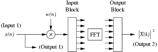
A block diagram representation of the spectrum analyzer you will implement in the lab, including
the required input and ouput locations, can be found depicted in Figure 1.8.
Figure 1.8.
FFT-based spectrum analyzer
Lab 4: Prelab*
MATLAB Exercise
Since the DFT is a sampled version of the spectrum of a digital signal, it has certain sampling
effects. To explore these sampling effects more thoroughly, we consider the effect of multiplying
the time signal by different window functions and the effect of using zero-padding to increase the
length (and thus the number of sample points) of the DFT. Using the following MATLAB script as
an example, plot the squared-magnitude response of the following test cases over the digital
frequencies
.
1. rectangular window with no zero-padding
2. hamming window with no zero-padding
3. rectangular window with zero-padding by factor of four ( i.e. , 1024-point FFT)
4. hamming window window with zero-padding by factor of four
Window sequences can be generated in MATLAB by using the boxcar and hamming functions.
1 N = 256; % length of test signals
2 num_freqs = 100; % number of frequencies to test
3
4 % Generate vector of frequencies to test
5
6 omega = pi/8 + [0:num_freqs-1]'/num_freqs*pi/4;
7
8 S = zeros(N,num_freqs); % matrix to hold FFT results
9
10
11 for i=1:length(omega) % loop through freq. vector
12 s = sin(omega(i)*[0:N-1]'); % generate test sine wave
13 win = boxcar(N); % use rectangular window
14 s = s.*win; % multiply input by window
15 S(:,i) = (abs(fft(s))).^2; % generate magnitude of FFT
16 % and store as a column of S
17 end
18
19 clf;
20 plot(S); % plot all spectra on same graph
21
Make sure you understand what every line in the script does. What signals are plotted?
You should be able to describe the tradeoff between mainlobe width and sidelobe behavior for the
various window functions. Does zero-padding increase frequency resolution? Are we getting
something for free? What is the relationship between the DFT, X[ k] , and the DTFT, X( ω) , of a sequence x[ n] ?
Lab 4: Lab*
Implementation
As this is your first experience with the C environment, you will have the option to add most of
the required code in C or assembly. A C skeleton will provide access to input samples, output
samples, and interrupt handling code. You will add code to transfer the inputs and outputs (in
blocks at a time), apply a hamming window, compute the magnitude-squared spectrum, and
include a trigger pulse. After the hamming window is created, either an assembly or C module that
bit reverses the input and performs an FFT calculation is called.
As your spectrum analyzer works on a block of samples at a time, you will need to use interrupts
to pause your processing while samples are transferred from/to the CODEC (A/D and D/A) buffer.
Fortunately, the interrupt handling routines have been written for you in a C shell program
available at v:\ece420\54x\dspclib\lab4main.c and the core code.
Interrupt Basics
Interrupts are an essential part of the operation of any microprocessor. They are particularly
important in embedded applications where DSPs are often used. Hardware interrupts provide a
way for interacting with external devices while the processor executes code. For example, in a key
entry system, a key press would generate a hardware interrupt. The system code would then jump
to a specified location in program memory where a routine could process the key input. Interrupts
provide an alternative to polling. Instead of checking for key presses at a predetermined rate
(requires a clock), the system could be busy executing other code. On the TI-C54x DSP, interrupts
provide a convenient way to transfer blocks of data to/from the CODEC in a timely fashion.
Interrupt Handling
The lab4main.c code and the core code are intended to make your interaction with the
hardware much simpler. As there was a core file for working in the assembly environment (Labs
0-3), there is a core file for the C environment (V:\ece420\54x\dspclib\core.asm) which handles
the interrupts from the CODEC (A/D and D/A) and the serial port. Here, we will describe the
important aspects of the core code necessary to complete the assignment.
At the heart of the hardware interaction is the auto-buffering serial port. In the auto-buffering
serial mode, the TI-C54x processor is able to do processing uninterrupted while samples are
transferred to/from a buffer of length BlockLen=64 samples. However, the spectrum analyzer to
be implemented in this lab works over a block of N=1024 samples. If it were possible to compute
a 1024-point FFT in the sample time of one BlockLen, then no additional interrupt handling
routines would be necessary. Samples could be collected in a 1024-length buffer and a 1024-point
FFT could be computed uninterrupted while the auto-buffering buffer fills. Unfortunately, the
DSP is not fast enough to accomplish this task.
We now provide an explanation of the shell C program lab4main.c listed in Appendix A. The lab4main.c file contains the function interrupt void irq and a main program. The
main program is an infinite loop over blocks of N=1024 samples. Note that while the DSP is
executing instructions in this loop, interrupts occur every BlockLen samples. Inside the infinite
loop, you will insert code to do the operations which follow. Although each of these operations
may be performed in C or assembly, we suggest you follow the guidelines suggested.
1. Transfer inputs and outputs (C)
2. Apply a Hamming Window (C/assembly)
3. Bit-reverse the input (C and assembly)
4. Apply an N -point FFT (C and assembly)
5. Compute the magnitude-squared spectrum (C/assembly)
6. Include a trigger pulse (C/assembly)
The function WaitAudio is an assembly function in the core code which handles the CODEC
interrupts. An interrupt from the CODEC occurs every BlockLen samples. The
SetAudioInterrupt(irq) call in the main program tells the core code to jump to the irq
function when an interrupt occurs. In the irq function, BlockLen samples of the A/D input in
Rcvptr (channel 1) are written to a length N inputs buffer, and BlockLen of the output
samples in the outputs buffer are written to the D/A output via Xmitptr on channel 2. In C,
pointers may be used as array names so that Xmitptr[0] is the first word pointed to by
Xmitptr. As in the assembly core, the input samples are not in consecutive order. The right and
left inputs are offset from Rcvptr respectively by 4 i and 4 i+2 , i=0 , …, BlockLen−1 . The six
output channels are accessed consecutively as offsets from Xmitptr. On channel 1 of the output,
the input is echoed out. You are to fill the buffer outputs with the windowed magnitude-
squared FFT values by performing the operations listed above.
In the main code, the while(!input_full); loop waits for N samples to collect in the
inputs buffer. Next, the N inputs and outputs must be transferred. You are to write this portion
of code. This portion of code is to be done first, within BlockLen sample times; otherwise the
first BlockLen of samples of output would not be available on time. Once this loop is finished,
the lengthy processing of the FFT can continue. During this processing, the DSP is interrupted
every BlockLen samples to transfer samples. Once this processing is over, the infinite loop
returns to while(!input_full); to wait for N samples to finish collecting.
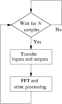
The flow diagram in Figure 1.9 summarizes the operation of the interrupt handling routine
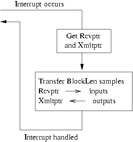
(b) interrupt handler
(a) main
Figure 1.9.
Overall program flow of the main function and the interrupt handling function.
Assembly FFT Routine
As the list of operations indicates, bit-reversal and FFT computation are to be done in both C and
assembly. For the assembly version, make sure that the line defining C_FFT is commented in
lab4main.c. We are providing you with a shell assembly file, available at
v:\ece420\54x\dspclib\c_fft_given.asm and shown in Appendix B, containing
many useful declarations and some code. The code for performing bit-reversal and other
declarations needed for the FFT routine are also provided in this section. However, we would like
you to enter this code manually, as you will be expected to understand its operation.
The assembly file c_fft_given.asm contains two main parts, the data section starting with
.sect ".data" and the program section starting with .sect ".text". Every function and
variable accessed in C must be preceded by a single underscore _ in assembly and a .global
_name must be placed in the assembly file for linking. In this example, bit_rev_fft is an
assembly function called from the C program with a label _bit_rev_fft in the text portion of
the assembly file and a .global _bit_rev_fft declaration. In each assembly function, the
macro ENTER_ASM is called upon entering and LEAVE_ASM is called upon exiting. These macros
are defined in v:\ece420\54x\dspclib\core.inc. The ENTER_ASM macro saves the
status registers and AR1, AR6, and AR7 when entering a function as required by the register use
conventions. The ENTER_ASM macro also sets the status registers to the assembly conventions we
have been using (i.e, FRCT=1 for fractional arithmetic and CPL=0 for DP referenced addressing).
The LEAVE_ASM macro just restores the saved registers.
Parameter Passing
The parameter passing convention between assembly and C is simple for single input, single
output assembly functions. From a C program, the input to an assembly program is in the low part
of accumulator A with the output returned in the same place. When more than one parameter is
passed to an assembly function, the parameters are passed on the stack (see the core file
description for more information). We suggest that you avoid passing or returning more than one
parameter. Instead, use global memory addresses to pass in or return more than one parameter.
Another alternative is to pass a pointer to the start of a buffer intended for passing and returning
parameters.
Registers Modified
When entering and leaving an assembly function, the ENTER_ASM and LEAVE_ASM macros
ensure that certain registers are saved and restored. Since the C program may use any and all
registers, the state of a register cannot be expected to remain the same between calls to assembly
function(s). Therefore, any information that needs to be preserved across calls to an assembly
function must be saved to memory!
Now, we explain how to use the FFT routine provided by TI for the C54x. The FFT routine
fft.asm located in v:\ece420\54x\dsplib\ computes an in-place, complex FFT. The
length of the FFT is defined as a label K_FFT_SIZE and the algorithm assumes that the input
starts at data memory location _fft_data. To have your code assemble for an N -point FFT,
you will have to include the following label definitions in your assembly code.
N .set 1024
K_FFT_SIZE .set N ; size of FFT
K_LOGN .set 10 ; number of stages (log_2(N))
In addition to defining these constants, you will have to include twiddle-factor tables for the FFT.
These tables (twiddle1 and twiddle2) are available in the shared directory v:\ece420\54x\dsplib\. Note that the tables are each N points long representing values
from 0 to just shy of 180 degrees and must be accessed using a circular pointer. To include these
tables at the proper location in memory with the appropriate labels referenced by the FFT, use the
following
.sect ".data"
.align 1024
sine .copy "v:\ece420\54x\dsplib\twiddle1"
.align 1024
cosine .copy "v:\ece420\54x\dsplib\twiddle2"
The FFT provided requires that the input be in bit-reversed order, with alternating real and
imaginary components. Bit-reversed addressing is a convenient way to order input x[ n] into a FFT
so that the output X( k) is in sequential order ( i.e. X(0) , X(1) , …, X( N−1) for an N -point FFT).
The following table illustrates the bit-reversed order for an eight-point sequence.
Table 1.2.
Input Order Binary Representation Bit-Reversed Representation Output Order
0
000
000
0
1
001
100
4
2
010
010
2
3
011
110
6
4
100
001
1
5
101
101
5
6
110
011
3
7
111
111
7
The following routine performs the bit-reversed reordering of the input data. The routine assumes
that the input is stored in data memory starting at the location labeled _bit_rev_data, which
must be aligned to the least power of two greater than the input buffer length, and consists of
alternating real and imaginary parts. Because our input data is going to be purely real in this lab,
you will have to make sure that you set the imaginary parts to zero by zeroing out every other
memory location.
1 bit_rev:
2 STM #_bit_rev_data,AR3 ; AR3 -> original input
3 STM #_fft_data,AR7 ; AR7 -> data processing buffer
4 MVMM AR7,AR2 ; AR2 -> bit-reversed data
5 STM #K_FFT_SIZE-1,BRC
6 RPTBD bit_rev_end-1
7 STM #K_FFT_SIZE,AR0 ; AR0 = 1/2 size of circ buffer
8 MVDD *AR3+,*AR2+
9 MVDD *AR3-,*AR2+
10 MAR *AR3+0B
11 bit_rev_end:
12 NOP
13 RET
As mentioned, in the above code _bit_rev_data is a label indicating the start of the input data
and _fft_data is a label indicating the start of a circular buffer where the bit-reversed data will
be written. Note that although AR7 is not used by the bit-reversed routine directly, it is used
extensively in the FFT routine to keep track of the start of the FFT data space.
In general, to have a pointer index memory in bit-reversed order, the AR0 register needs to be set
to one-half the length of the circular buffer; a statement such as ARx+0B is used to move the ARx
pointer to the next location. For more information regarding the bit-reversed addressing mode,
refer to page 5-18 in the TI-54x CPU and Peripherals manual [url]. Is it possible to bit-reverse a buffer in place? For a diagram of the ordering of the data expected by the FFT routine, see Figure
4-10 in the TI-54x Applications Guide [url]. Note that the FFT code uses all the pointers available and does not restore the pointers to their original values.
C FFT Routine
A bit-reversing and FFT routine have also been provided in lab4fft.c, listed in Appendix C.
Again, make sure you understand how the bit reversal is taking place. In lab4main.c, the
line defining C_FFT must not be commented for use of the C FFT routine. The sine tables
(twiddle factors) are located in sinetables.h. This fft requires its inputs in two buffers, the real buffer real and the imaginary buffer imag, and the output is placed in the same buffers. The
length of the FFT, N, and logN are defined in lab4.h, which is also listed in Appendix C.
When experimenting with the C FFT make sure you modify these length values instead of the
ones in the assembly code and lab4main.c!
Creating the Window
As mentioned, you will be using the FFT to compute the spectrum of a windowed input. For your
implementation you will need to create a 1024-point Hamming window. First, create a Hamming
window in matlab using the function hamming. For the assembly FFT, use save_coef to save
the window to a file that can then be included in your code with the .copy directive. For the C
FFT, use the matlab function write_intvector_headerfile with name set to 'window'
and elemperline set to 8 to create the header file that is included in lab4main.c.
Displaying the Spectrum
Once the DFT has been computed, you must calculate the squared magnitude of the spectrum for
display.
()
(| X( k)|)2=(ℜ( X( k)))2+(ℑ( X( k)))2
You may find the assembly instructions squr and squra useful in implementing Equation.
Because the squared magnitude is always nonnegative, you can replace one of the magnitude
values with a -1.0 as a trigger pulse for display on the oscilloscope. This is easily performed by
replacing the DC term ( k=0 ) with a -1.0 when copying the magnitude values to the output buffer.
The trigger pulse is necessary for the oscilloscope to lock to a specific point in the spectrum and
keep the spectrum fixed on the scope.
Intrinsics
If you are planning on writing some of the code in C, then you may be forced to use intrinsics.
Intrinsic instructions provide a way to use assembly instructions directly in C. An example of an
intrinsic instruction is bit_rev_data[0]=_smpyr(bit_rev_data[0],window[0])
which performs the assembly signed multiply round instruction. You may also find the _lsmpy
instruction useful. For more information on intrinsics, see page 6-22 of the TI-C54x Optimizing
C/C++ Compiler User's Guide [url].
The following lines of code were borrowed from the C FFT to serve as an example of arithmetic
operations in C. Save this code in a file called mathex.c and compile this file. Look at the
resulting assembly file and investigate the differences between each block. Be sure to reference
the compiler user's guide to find out what the state of the FRCT and OVM bits are. Does each
block work properly for all possible values?
void main(void)
{
int s1, s2;