ECE 320 Spring 2004 by Mark Butala, et al - HTML preview
Download the book in PDF, ePub for a complete version.
ECE 320 Spring 2004
Collection edited by: Robert Morrison and Jason Laska
Content authors: Mark Butala, Jason Laska, Douglas Jones, Swaroop Appadwedula, Matthew
Berry, Mark Haun, Jake Janevitz, Michael Kramer, Dima Moussa, Daniel Sachs, Brian Wade,
Robert Morrison, Matt Kleffner, Michael Frutiger, Arjun Kulothungun, and Richard Cantzler
Online: < http://cnx.org/content/col10225/1.12>
This selection and arrangement of content as a collection is copyrighted by Robert Morrison and Jason Laska.
It is licensed under the Creative Commons Attribution License: http://creativecommons.org/licenses/by/1.0
Collection structure revised: 2004/08/24
For copyright and attribution information for the modules contained in this collection, see the " Attributions" section at the end of the collection.
ECE 320 Spring 2004
Table of Contents
Step 4: Verify filter execution
Step 5: Re-assemble and re-run with new filter
Step 6: Check filter response in MATLAB
Step 7: Create new filter in MATLAB and verify
Step 8: Modify filter coefficients in memory
Step 9: Test-vector simulation
Part 1: Single-Channel FIR Filter
Part 2: Dual-Channel FIR Filters
Part 3: Alternative Single-Channel FIR Implementation
Real-time rate change and MATLAB interface (Optional)
Preparing for processor implementation
Filter-Coefficient Quantization
Quantizing coefficients in MATLAB
Pseudo-Noise Sequence Generator
Viewing the signal spectrum on the VSA
Adaptive Filtering: LMS Algorithm
Audio Effects: Real-Time Control with the Serial Port
Feedback system implementation
MATLAB interface implementation
Audio Effects: Using External Memory
Fixed-length delay implementation
Communications: Using Direct Digital Synthesis
Frequency Modulation (FM) Radio Exercise
Digital Receiver: Carrier Recovery
Numerically controlled oscillator
Digital Receivers: Symbol-Timing Recovery for QPSK
Essential documentation for the 6000 series TI DSP
Video Processing Part 1: Introductory Exercise
Video Processing Part 2: Grayscale and Color
Video Processing Part 3: Memory Management
The INPUT and OUTPUT buffers and Main.c Details
Creating and Destroying Streams
Surround Sound: Passive Encoding and Decoding
Surround Sound: Chamberlin Filters
Speech Processing: LPC Exercise in MATLAB
Speech Processing: Theory of LPC Analysis and Synthesis
Speech Processing: LPC Exercise on TI TMS320C54x
Chapter 1. Weekly Labs
1.1. Lab 0
Lab 0: Hardware Introduction*
Introduction
This exercise introduces the hardware and software used in testing a simple DSP system. When
you complete it, you should be comfortable with the basics of testing a simple real-time DSP
system with the debugging environment you will use throughout the course. First, you will
connect the laboratory equipment and test a real-time DSP system with pre-written code to
implement an eight-tap (eight coefficient) finite impulse response ( FIR) filter. With a working
system available, you will then begin to explore the debugging software used for downloading,
modifying, and testing code. Finally, exercises are included to refresh your familiarity with
MATLAB.
Lab Equipment
This exercise assumes you have access to a laboratory station equipped with a Texas Instruments
TMS320C549 digital signal processor chip mounted on a Spectrum Digital TMS320LC54x
evaluation board. The DSP evaluation module should be connected to a PC running Windows and
will be controlled using the PC application Code Composer Studio, a debugger and development
environment. Mounted on top of each DSP evaluation board is a Spectrum Digital surround-sound
module employing a Crystal Semiconductor CS4226 codec. This board provides two analog input
channels and six analog output channels at the CD sample rate of 44.1 kHz. The DSP board can
also communicate with user code or a terminal emulator running on the PC via a serial data
interface.
In addition to the DSP board and PC, each laboratory station should also be equipped with a
function generator to provide test signals and an oscilloscope to display the processed waveforms.
Step 1: Connect cables
Use the provided BNC cables to connect the output of the function generator to input channel 1 on
the DSP evaluation board. Connect output channels 1 and 2 of the board to channels 1 and 2 of the
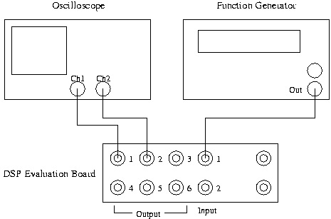
oscilloscope. The input and output connections for the DSP board are shown in Figure 1.1.
Figure 1.1. Example Hardware Setup
Note that with this configuration, you will have only one signal going into the DSP board and two
signals coming out. The output on channel 1 is the filtered input signal, and the output on channel
2 is the unfiltered input signal. This allows you to view the raw input and filtered output
simultaneously on the oscilloscope. Turn on the function generator and the oscilloscope.
Step 2: Log in
Use the network ID and password provided to log into the PC at your laboratory station.
When you log in, two shared networked drives should be mapped to the computer: the W: drive,
which contains your own private network work directory, and the V: drive, where the necessary
files for ECE 420 are stored. Be sure to save any files that you use for the course to the W: drive.
Temporary files may be stored in the C:\TEMP directory; however, since files stored on the C:
drive are accessible to any user, are local to each computer, and may be erased at any time, do not
store course files on the C: drive. On the V: drive, the directories
v:\ece420\54kx\dsplib\ and c:\ece420\54x\dsptools\ contain the files necessary
to assemble and test code on the TI DSP evaluation boards.
Although you may want to work exclusively in one or the other of lab-partners' network account,
you should be sure that both partners have copies of the lab assignment assembly code.
Warning
Not having the assembly code during a quiz because "it's on my partner's account" is NOT a
valid excuse!
For copying between partners' directory on W: or for working outside the lab, FTP access to your
files is available at ftp://elalpha.ece.uiuc.edu.
The Development Environment
The evaluation board is controlled by the PC through the JTAG interface (XDS510PP) using the
application Code Composer Studio. This development environment allows the user to download,
run, and debug code assembled on the PC. Work through the steps below to familiarize yourself
with the debugging environment and real-time system using the provided FIR filter code (Steps 3,
4 and 5), then verify the filter's frequency response with the subsequent MATLAB exercises
(Steps 6 and 7).
Step 3: Assemble filter code
Before you can execute and test the provided FIR filter code, you must assemble the source file.
First, bring up a DOS prompt window and create a new directory to hold the files, and then copy
them into your directory:
w:
mkdir lab0
cd lab0
copy v:\ece420\54x\dsplib\filter.asm .
copy v:\ece420\54x\dsplib\coef.asm .
Next, assemble the filter code by typing asm filter at the DOS prompt. The assembling
process first includes the FIR filter coefficients (stored in coef.asm) into the assembly file
filter.asm, then compiles the result to produce an output file containing the executable binary
code, filter.out.
Step 4: Verify filter execution
With your filter code assembled, double-click on the Code Composer icon to open the debugging
environment. Before loading your code, you must reset the DSP board and initialize the processor
mode status register ( PMST). To reset the board, select the Reset option from the Debug
menu in the Code Composer application.
Once the board is reset, select the CPU Registers option from the View menu, then select
CPU Register. This will open a sub-window at the bottom of the Code Composer application
window that displays several of the DSP registers. Look for the PMST register; it must be set to
the hexadecimal value FFE0 to have the DSP evaluation board work correctly. If it is not set
correctly, change the value of the PMST register by double-clicking on the value and making the
appropriate change in the Edit Register window that comes up.
Now, load your assembled filter file onto the DSP by selecting Load Program from the File
menu. Finally, reset the DSP again, and execute the code by selecting Run from the Debug menu.
The program you are running accepts input from input channel 1 and sends output waveforms to
output channels 1 and 2 (the filtered signal and raw input, respectively). Note that the "raw input"
on output channel 2 may differ from the actual input on input channel 1, because of distortions
introduced in converting the analog input to a digital signal and then back to an analog signal. The
A/D and D/A converters on the six-channel surround board operate at a sample rate of 44.1 kHz
and have an anti-aliasing filter and an anti-imaging filter, respectively, that in the ideal case
would eliminate frequency content above 22.05 kHz. The converters on the six-channel board are
also AC coupled and cannot pass DC signals. On the basis of this information, what differences
do you expect to see between the signals at input channel 1 and at output channel 2?
Set the amplitude on the function generator to 1.0 V peak-to-peak and the pulse shape to
sinusoidal. Observe the frequency response of the filter by sweeping the input signal through the
relevant frequency range. What is the relevant frequency range for a DSP system with a sample
rate of 44.1 kHz?
Based on the frequency response you observe, characterize the filter in terms of its type (e.g., low-
pass, high-pass, band-pass) and its -6 dB (half-amplitude) cutoff frequency (or frequencies). It
may help to set the trigger on channel 2 of the oscilloscope since the signal on channel 1 may go
to zero.
Step 5: Re-assemble and re-run with new filter
Once you have determined the type of filter the DSP is implementing, you are ready to repeat the
process with a different filter by including different coefficients during the assembly process.
Copy a second set of FIR coefficients over to your working directory with the following:
copy coef.asm coef1.asm
copy v:\ece420\54x\dsplib\coef2.asm coef.asm
You can now repeat the assembly and testing process with the new filter using the asm instruction
at the DOS prompt and repeating the steps required to execute the code discussed in Step 4.
Just as you did in Step 4, determine the type of filter you are running and the filter's -6 dB point by testing the system at various frequencies.
Step 6: Check filter response in MATLAB
In this step, you will use MATLAB to verify the frequency response of your filter by copying the
coefficients from the DSP to MATLAB and displaying the magnitude of the frequency response
using the MATLAB command freqz.
The FIR filter coefficients included in the file coef.asm are stored in memory on the DSP
starting at location (in hex) 0x1000, and each filter you have assembled and run has eight
coefficients. To view the filter coefficients as signed integers, select the Memory option from the
View menu to bring up a Memory Window Options box. In the appropriate fields, set the
starting address to 0x1000 and the format to 16-Bit Signed Int. Click "OK" to open a
memory window displaying the contents of the specified memory locations. The numbers along
the left-hand side indicate the memory locations.
In this example, the filter coefficients are placed in memory in decreasing order; that is, the last
coefficient, h[7] , is at location 0x1000 and the first coefficient, h[0] , is stored at 0x1007.
Now that you can find the coefficients in memory, you are ready to use the MATLAB command
freqz to view the filter's response. You must create a vector in MATLAB with the filter
coefficients to use the freqz command. For example, if you want to view the response of the
three-tap filter with coefficients -10, 20, -10 you can use the following commands in MATLAB:
h = [-10, 20, -10];
plot(abs(freqz(h)))
Note that you will have to enter eight values, the contents of memory locations 0x1000 through
0x1007, into the coefficient vector, h.
Does the MATLAB response compare with your experimental results? What might account for
any differences?
Step 7: Create new filter in MATLAB and verify
MATLAB scripts will be made available to you to aid in code development. For example, one of
these scripts allows you to save filter coefficients created in MATLAB in a form that can be
included as part of the assembly process without having to type them in by hand (a very useful
tool for long filters). These scripts may already be installed on your computer; otherwise,
download the files from the links as they are introduced.
First, have MATLAB gene