Fundamentals of Transportation by Michael Corbett, Adam Danczyk, et al - HTML preview
Download the book in PDF, ePub, Kindle for a complete version.
0 or 1), and we want to talk
about probabilities of choices
that range from 0 to 1. (If we
do a regression on 0s and 1s
we might measure for j a
probability of 1.4 or -0.2 of
taking an auto.) Further, the
distribution of the error terms
wouldn’t have appropriate statistical characteristics.
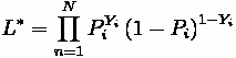
The MNL approach is to make a maximum likelihood estimate of this functional form. The
likelihood function is:
we solve for the estimated parameters
that max L*. This happens when:
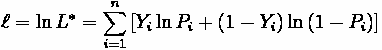
The log-likelihood is easier to work with, as the products turn to sums:
Consider an example adopted from John Bitzan’s Transportation Economics Notes. Let X be a binary variable that is gamma and 0 with probability (1- gamma). Then f(0) = (1- gamma) and f(1) = gamma. Suppose that we have 5 observations of X, giving the sample
{1,1,1,0,1}. To find the maximum likelihood estimator of gamma examine various values of gamma, and for these values determine the probability of drawing the sample {1,1,1,0,1} If gamma takes the value 0, the probability of drawing our sample is 0. If gamma is 0.1, then the probability of getting our sample is: f(1,1,1,0,1) = f(1)f(1)f(1)f(0)f(1) =
0.1*0.1*0.1*0.9*0.1=0.00009. We can compute the probability of obtaining our sample over
Fundamentals of Transportation/Mode Choice
47
a range of gamma – this is our likelihood function. The likelihood function for n independent observations in a logit model is
where: Yi = 1 or 0 (choosing e.g. auto or not-auto) and Pi = the probability of observing Yi=1
The log likelihood is thus:
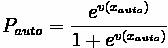
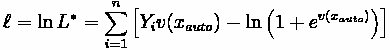
In the binomial (two alternative) logit model,
, so
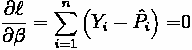
The log-likelihood function is maximized setting the partial derivatives to zero:
The above gives the essence of modern MNL choice modeling.
Independence of Irrelevant Alternatives (IIA)
Independence of Irrelevant Alternatives is a property of Logit, but not all Discrete Choice models. In brief, the implication of IIA is that if you add a mode, it will draw from present modes in proportion to their existing shares. (And similarly, if you remove a mode, its users will switch to other modes in proportion to their previous share). To see why this property may cause problems, consider the following example: Imagine we have seven modes in our
logit mode choice model (drive alone, carpool 2 passenger, carpool 3+ passenger, walk to transit, auto driver to transit (park and ride), auto passenger to transit (kiss and ride), and walk or bike). If we eliminated Kiss and Ride, a disproportionate number may use Park and Ride or carpool.
Consider another example. Imagine there is a mode choice between driving and taking a
red bus, and currently each has 50% share. If we introduce another mode, let's call it a blue bus with identical attributes to the red bus, the logit mode choice model would give each mode 33.3% of the market, or in other words, buses will collectively have 66.7% market
share. Logically, if the mode is truly identical, it would not attract any additional
passengers (though one can imagine scenarios where adding capacity would increase bus
mode share, particularly if the bus was capacity constrained.
There are several strategies that help with the IIA problem. Nesting of choices allows us to reduce this problem. However, there is an issue of the proper Nesting structure. Other
alternatives include more complex models (e.g. Mixed Logit) which are more difficult to
estimate.


Fundamentals of Transportation/Mode Choice
48
Consumers' Surplus
Topics not touched on include the “red bus, blue bus” problem; the use of nested models
(e.g., estimate choice between auto and transit, and then estimate choice between rail and bus transit); how consumers’ surplus measurements may be obtained; and model
estimation, goodness of fit, etc. For these topics see a textbook such as Ortuzar and
Willumsen (2001).
Returning to roots
The discussion above is based on the economist’s utility formulation. At the time MNL
modeling was developed there was some attention to psychologist's choice work (e.g.,
Luce’s choice axioms discussed in his Individual Choice Behavior, 1959). It has an analytic side in computational process modeling. Emphasis is on how people think when they make
choices or solve problems (see Newell and Simon 1972). Put another way, in contrast to
utility theory, it stresses not the choice but the way the choice was made. It provides a conceptual framework for travel choices and agendas of activities involving considerations of long and short term memory, effectors, and other aspects of thought and decision
processes. It takes the form of rules dealing with the way information is searched and acted on. Although there is a lot of attention to behavioral analysis in transportation work, the best of modern psychological ideas are only beginning to enter the field. (e.g. Golledge, Kwan and Garling 1984; Garling, Kwan, and Golledge 1994).
Examples
Example 1: Mode Choice Model
Problem:
You are given this mode choice model
Where:
•
= cost of mode (cents) / wage rate (in cents per minute)
•
= travel time in-vehicle (min)
•
= travel time out-of-vehicle (min)
•
= mode specific dummies: (dummies take the value of 1 or 0)
•
= driving,
•
= transit with walk access, [base mode]
•
= transit with auto access,
•
= carpool
With these inputs:
''
Driving
Walk Connect
Auto Connect
Carpool
Transit
Transit
t = travel time in-vehicle (min)
10
30
15
12


Fundamentals of Transportation/Mode Choice
49
t0 = travel time out-of-vehicle (min)
0
15
10
3
= driving,
1
0
0
0
= transit with walk access, [base
0
1
0
0
mode]
= transit with auto access,
0
0
1
0
= carpool
0
0
0
1
COST
25
100
100
150
WAGE
60
60
60
60
What are the resultant mode shares?
Solution:
Outputs
1: Driving
2: Walk-connect transit
3: Auto-connect transit
4: Carpool
Sum
Utilities
-1.26
-2.09
-3.30
-3.58
EXP(V)
0.28
0.12
0.04
0.03
P(V)
59.96%
26.31%
7.82%
5.90%
100%
Interpretation
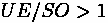
Value of Time:
(in 1967 $, when the wage rate was about $2.85/hour)
implication, if you can improve the travel time (by more buses, less bottlenecks, e.g.) for less than $1.10/hour/person, then it is socially worthwhile.
Example 2: Mode Choice Model Interpretation
Case 1
''
Bus
Car
Parameter
Tw
10 min
5 min
-0.147
Tt
40 min
20 min
-0.0411
C
$2
$1
-2.24
Car always wins (independent of parameters as long as all are < 0)
Case 1


Fundamentals of Transportation/Mode Choice
50
''
Bus
Car
Parameter
Tw
5 min
5 min
-0.147
Tt
40 min
20 min
-0.0411
C
$2
$4
-2.24
Results
-6.86
-10.51
Under observed parameters, bus always wins, but not necessarily under all parameters.
It is important to note that individuals differ in parameters. We could introduce
socio-economic and other observable characteristics as well as a stochastic error term to make the problem more realistic.
Sample Problem
• Problem ( Solution ) Variables
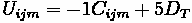
•
- Utility of traveling from i to j by mode m
•
= mode specific dummies: (dummies take the value of 1 or 0)
•
= Probability of mode m
•
= cost of mode (cents) / wage rate (in cents per minute)
•
= travel time in-vehicle (min)
•
= travel time out-of-vehicle (min)
•
= mode specific dummies: (dummies take the value of 1 or 0)
Abbreviations
• WCT - walk connected transit
• ADT - auto connect transit (drive alone/park and ride)
• APT - auto connect transit (auto passenger/kiss and ride)
• AU1 - auto driver (no passenger)
• AU2 - auto 2 occupants
• AU3+ - auto 3+ occupants
• WK/BK - walk/bike
• IIA - Independence of Irrelevant Alternatives
Key Terms
• Mode choice
• Logit
• Probability
• Independence of Irrelevant Alternatives (IIA)
• Dummy Variable (takes value of 1 or 0)


Fundamentals of Transportation/Mode Choice
51
References
• Garling, Tommy Mei Po Kwan, and Reginald G. Golledge. Household Activity Scheduling,
Transportation Research, 22B, pp. 333-353. 1994.
• Golledge. Reginald G., Mei Po Kwan, and Tommy Garling, “Computational Process
Modeling of Household Travel Decisions,” Papers in Regional Science, 73, pp. 99-118.
1984.
• Lancaster, K.J., A new approach to consumer theory. Journal of Political Economy, 1966.
74(2): p. 132-157.
• Luce, Duncan R. (1959). Individual choice behavior, a theoretical analysis. New York,
Wiley.
• Newell, A. and Simon, H. A. (1972). Human Problem Solving. Englewood Cliffs, NJ:
Prentice Hall.
• Ortuzar, Juan de Dios and L. G. Willumsen’s Modelling Transport. 3rd Edition. Wiley and Sons. 2001,
• Thurstone, L.L. (1927). A law of comparative judgement. Psychological Review, 34,
278-286.
• Warner, Stan 1962 Strategic Choice of Mode in Urban Travel: A Study of Binary Choice
Fundamentals of Transportation/
Mode Choice/Problem
Problem:
You are given the following mode choice model.
Where:
•
= travel cost between and by mode
•
= dummy variable (alternative specific constant) for transit
and Travel Times
Auto Travel Times
Origin\Destination
Dakotopolis
New Fargo
Dakotopolis
5
7
New Fargo
7
5
Transit Travel Times
Origin\Destination
Dakotopolis
New Fargo
Dakotopolis
10
15
New Fargo
15
8


Fundamentals of Transportation/Mode Choice/Problem
52
A. Using a logit model, determine the probability of a traveler driving.
B. Using the results from the previous problem (#2), how many car trips will there be?
• Solution
Fundamentals of Transportation/
Mode Choice/Solution
Problem:
You are given the following mode choice model.
Where:
•
= travel cost between and by mode
•
= dummy variable (alternative specific constant) for transit
Auto Travel Times
Origin\Destination
Dakotopolis
New Fargo
Dakotopolis
5
7
New Fargo
7
5
Transit Travel Times
Origin\Destination
Dakotopolis
New Fargo
Dakotopolis
10
15
New Fargo
15
8
Solution:
Part A
A. Using a logit model, determine the probability of a traveler driving.
Solution Steps
1. Compute Utility for Each Mode for Each Cell
2. Compute Exponentiated Utilities for Each Cell
3. Sum Exponentiated Utilities
4. Compute Probability for Each Mode for Each Cell
5. Multiply Probability in Each Cell by Number of Trips in Each Cell
Fundamentals of Transportation/Mode Choice/Solution
53
Auto Utility:
Origin\Destination
Dakotopolis
New Fargo
Dakotopolis
-5
-7
New Fargo
-7
-5
Transit Utility:
Origin\Destination
Dakotopolis
New Fargo
Dakotopolis
-5
-10
New Fargo
-10
-3
Origin\Destination
Dakotopolis
New Fargo
Dakotopolis
0.0067
0.0009
New Fargo
0.0009
0.0067
Origin\Destination
Dakotopolis
New Fargo
Dakotopolis
0.0067
0.0000454
New Fargo
0.0000454
0.0565
Sum:
Origin\Destination
Dakotopolis
New Fargo
Dakotopolis
0.0134
0.0009454
New Fargo
0.0009454
0.0498
P(Auto) =
Origin\Destination
Dakotopolis
New Fargo
Dakotopolis
0.5
0.953
New Fargo
0.953
0.12
P(Transit) =
Origin\Destination
Dakotopolis
New Fargo
Dakotopolis
0.5
0.047
New Fargo
0.047
0.88
Part B
B. Using the results from the previous problem (#2), how many car trips will there be?
Recall


Fundamentals of Transportation/Mode Choice/Solution
54
Total Trips
Origin\Destination
Dakotopolis
New Fargo
Dakotopolis
9395
5606
New Fargo
6385
15665
Total Trips by Auto =
Origin\Destination
Dakotopolis
New Fargo
Dakotopolis
4697
5339
New Fargo
6511
1867
Fundamentals of Transportation/
Route Choice
Route assignment, route choice, or traffic assignment concerns the selection of routes (alternative called paths) between origins and destinations in transportation networks. It is
the fourth step in the conventional transportation forecasting model, following Trip
Generation, Destination Choice, and Mode Choice. The zonal interchange analysis of trip distribution provides origin-destination trip tables. Mode choice analysis tells which
travelers will use which mode. To determine facility needs and costs and benefits, we need to know the number of travelers on each route and link of the network (a route is simply a chain of links between an origin and destination). We need to undertake traffic (or trip) assignment. Suppose there is a network of highways and transit systems and a proposed
addition. We first want to know the present pattern of travel times and flows and then what would happen if the addition were made.
Link Performance Function
The cost that a driver imposes on others is called the marginal cost. However, when making decisions, a driver only faces his own cost (the average cost) and ignores any costs imposed on others (the marginal cost).
•
•
Fundamentals of Transportation/Route Choice
55
Can Flow Exceed Capacity?
On a link, the capacity is thought of as “outflow.” Demand is inflow.
If inflow > outflow for a period of time, there is queueing (and delay).
For Example, for a 1 hour period, if 2100 cars arrive and 2000 depart, 100 are still there.
The link performance function tries to represent that phenomenon in a simple way.
Wardrop's Principles of Equilibrium
User Equilibrium
Each user acts to minimize his/her own cost, subject to every other user doing the same.
Travel times are equal on all used routes and lower than on any unused route.
System optimal
Each user