Fundamentals of Transportation by Michael Corbett, Adam Danczyk, et al - HTML preview
Download the book in PDF, ePub, Kindle for a complete version.
Office of Management and Budget (OMB) – 1977
Throughout the next few decades, the federal government continued to demand improved
benefit-cost analysis with the aim of encouraging transparency and accountability.
Approximately 12 years after the adoption of the PPBS system, the Bureau of the Budget
was renamed the Office of Management and Budget (OMB). The OMB formally adopted a
system that attempts to incorporate benefit-cost logic into budgetary decisions. This came from the Zero-Based Budgeting system set up by Jimmy Carter when he was governor of
Georgia (Gramlich, 1981).
Recent Developments
Executive Order 12292, issued by President Reagan in 1981, required a regulatory impact
analysis (RIA) for every major governmental regulatory initiative over $100 million. The RIA is basically a benefit-cost analysis that identifies how various groups are affected by the policy and attempts to address issues of equity (Boardman, 1996).
According to Robert Dorfman, (Dorfman, 1997) most modern-day benefit-cost analyses
suffer from several deficiencies. The first is their attempt “to measure the social value of all the consequences of a governmental policy or undertaking by a sum of dollars and cents”.
Specifically, Dorfman mentions the inherent difficultly in assigning monetary values to
human life, the worth of endangered species, clean air, and noise pollution. The second
shortcoming is that many benefit-cost analyses exclude information most useful to decision makers: the distribution of benefits and costs among various segments of the population.
Government officials need this sort of information and are often forced to rely on other sources that provide it, namely, self-seeking interest groups. Finally, benefit-cost reports are often written as though the estimates are precise, and the readers are not informed of the range and/or likelihood of error present.
The Clinton Administration sought proposals to address this problem in revising Federal
benefit-cost analyses. The proposal required numerical estimates of benefits and costs to be made in the most appropriate unit of measurement, and “specify the ranges of predictions and shall explain the margins of error involved in the quantification methods and in the estimates used” (Dorfman, 1997). Executive Order 12898 formally established the concept
of Environmental Justice with regards to the development of new laws and policies, stating they must consider the “fair treatment for people of all races, cultures, and incomes.” The order requires each federal agency to identify and address “disproportionately high and
adverse human health or environmental effects of its programs, policies and activities on minority and low-income populations.”
Fundamentals of Transportation/Evaluation
71
Probabilistic Benefit-Cost Analysis
In recent years there has been a push
for the integration of sensitivity
analyses of possible outcomes of public
investment projects with open
discussions of the merits of
assumptions used. This “risk analysis”
process has been suggested by
Flyvbjerg (2003) in the spirit of
encouraging more transparency and
public involvement in decision-aking.
The Treasury Board of Canada’s
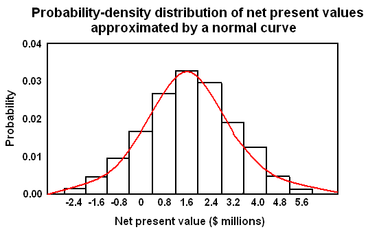
Probability-density distribution of net present values
Benefit-Cost Analysis Guide recognizes
approximated by a normal curve. Source: Treasury Board of
that implementation of a project has a
Canada, Benefit-Cost Analysis Guide, 1998
probable range of benefits and costs. It
posits that the “effective sensitivity” of
an outcome to a particular variable is
determined by four factors:
• the responsiveness of the Net
Present Value (NPV) to changes in
the variable;
• the magnitude of the variable's
range of plausible values;
• the volatility of the value of the
variable (that is, the probability that
the value of the variable will move
within that range of plausible
values); and
• the degree to which the range or
volatility of the values of the variable
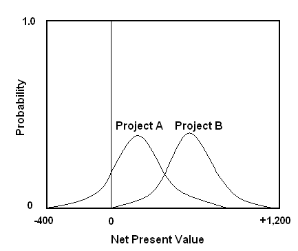
Probability distribution curves for the NPVs of projects A
can be controlled.
and B. Source: Treasury Board of Canada, Benefit-Cost
It is helpful to think of the range of
Analysis Guide, 1998.
probable outcomes in a graphical
sense, as depicted in Figure 1 (probability versus NPV).
Once these probability curves are generated, a comparison of different alternatives can also be performed by plotting each one on the same set of ordinates. Consider for example, a
comparison between alternative A and B (Figure 2).
Fundamentals of Transportation/Evaluation
72
In Figure 2, the probability that any
specified positive outcome will be
exceeded is always higher for project B
than it is for project A. The decision
maker should, therefore, always prefer
project B over project A. In other
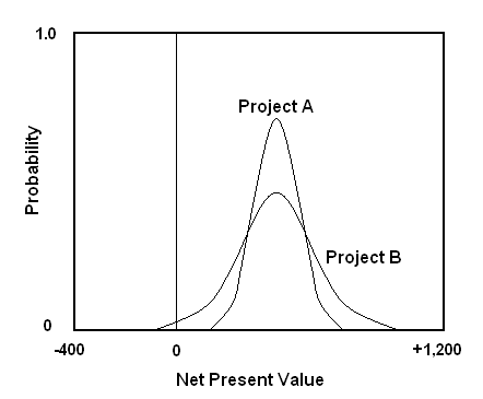
cases, an alternative may have a much
broader or narrower range of NPVs
compared to other alternatives (Figure
3).
Some decision-makers might be
attracted by the possibility of a higher
return (despite the possibility of
greater loss) and therefore might
choose project B. Risk-averse
Probability distribution curves for the NPVs of projects A
and B, where Project A has a narrower range of possible
decision-makers will be attracted by
NPVs. Source: Treasury Board of Canada, Benefit-Cost
the possibility of lower loss and will
Analysis Guide, 1998
therefore be inclined to choose project
A.
Discount rate
Both the costs and benefits flowing from an investment are spread over time. While some
costs are one-time and borne up front, other benefits or operating costs may be paid at
some point in the future, and still others received as a stream of payments collected over a long period of time. Because of inflation, risk, and uncertainty, a dollar received now is worth more than a dollar received at some time in the future. Similarly, a dollar spent today is more onerous than a dollar spent tomorrow. This reflects the concept of time preference that we observe when people pay bills later rather than sooner. The existence of real
interest rates reflects this time preference. The appropriate discount rate depends on what other opportunities are available for the capital. If simply putting the money in a
government insured bank account earned 10% per year, then at a minimum, no investment
earning less than 10% would be worthwhile. In general, projects are undertaken with those with the highest rate of return first, and then so on until the cost of raising capital exceeds the benefit from using that capital. Applying this efficiency argument, no project should be undertaken on cost-benefit grounds if another feasible project is sitting there with a higher rate of return.
Three alternative bases for the setting the government’s test discount rate have been
proposed:
1. The social rate of time preference recognizes that a dollar's consumption today will be more valued than a dollar's consumption at some future time for, in the latter case, the dollar will be subtracted from a higher income level. The amount of this difference per
dollar over a year gives the annual rate. By this method, a project should not be
undertaken unless its rate of return exceeds the social rate of time preference.
2. The opportunity cost of capital basis uses the rate of return of private sector investment, a government project should not be undertaken if it earns less than a private sector
investment. This is generally higher than social time preference.
Fundamentals of Transportation/Evaluation
73
3. The cost of funds basis uses the cost of government borrowing, which for various
reasons related to government insurance and its ability to print money to back bonds,
may not equal exactly the opportunity cost of capital.
Typical estimates of social time preference rates are around 2 to 4 percent while estimates of the social opportunity costs are around 7 to 10 percent.
Generally, for Benefit-Cost studies an acceptable rate of return (the government’s test rate) will already have been established. An alternative is to compute the analysis over a range of interest rates, to see to what extent the analysis is sensitive to variations in this factor. In the absence of knowing what this rate is, we can compute the rate of return (internal rate of return) for which the project breaks even, where the net present value is zero. Projects with high internal rates of return are preferred to those with low rates.
Determine a present value
The basic math underlying the idea of determining a present value is explained using a
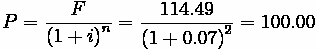
simple compound interest rate problem as the starting point. Suppose the sum of $100 is
invested at 7 percent for 2 years. At the end of the first year the initial $100 will have earned $7 interest and the augmented sum ($107) will earn a further 7 percent (or $7.49) in the second year. Thus at the end of 2 years the $100 invested now will be worth $114.49.
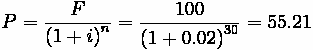
The discounting problem is simply the converse of this compound interest problem. Thus,
$114.49 receivable in 2 years time, and discounted by 7 per cent, has a present value of $100.
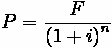
Present values can be calculated by the following equation:
(1)
where:
• F = future money sum
• P = present value
• i = discount rate per time period (i.e. years) in decimal form (e.g. 0.07)
• n = number of time periods before the sum is received (or cost paid, e.g. 2 years)
Illustrating our example with equations we have:
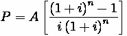
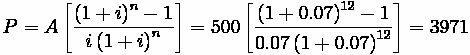
The present value, in year 0, of a stream of equal annual payments of $A starting year 1, is given by the reciprocal of the equivalent annual cost. That is, by:
(2)
where:
• A = Annual Payment
For example: 12 annual payments of $500, starting in year 1, have a present value at the middle of year 0 when discounted at 7% of: $3971

Fundamentals of Transportation/Evaluation
74
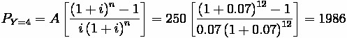
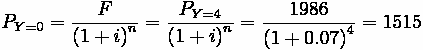
The present value, in year 0, of m annual payments of $A, starting in year n + 1, can be calculated by combining discount factors for a payment in year n and the factor for the
present value of m annual payments. For example: 12 annual mid-year payments of $250 in
years 5 to 16 have a present value in year 4 of $1986 when discounted at 7%. Therefore in year 0, 4 years earlier, they have a present value of $1515.
Evaluation criterion
Three equivalent conditions can tell us if a project is worthwhile
1. The discounted present value of the benefits exceeds the discounted present value of the costs
2. The present value of the net benefit must be positive.
3. The ratio of the present value of the benefits to the present value of the costs must be greater than one.
However, that is not the entire story. More than one project may have a positive net
benefit. From the set of mutually exclusive projects, the one selected should have the
highest net present value. We might note that if there are insufficient funds to carry out all mutually exclusive projects with a positive net present value, then the discount used in computing present values does not reflect the true cost of capital. Rather it is too low.
There are problems with using the internal rate of return or the benefit/cost ratio methods for project selection, though they provide useful information. The ratio of benefits to costs depends on how particular items (for instance, cost savings) are ascribed to either the
benefit or cost column. While this does not affect net present value, it will change the ratio of benefits to costs (though it cannot move a project from a ratio of greater than one to less than one).
Examples
Example 1: Benefit Cost Application
Problem:
This problem, adapted from Watkins (1996) [2], illustrates how a Benefit Cost
Analysis might be applied to a project such as a highway widening. The
improvement of the highway saves travel time and increases safety (by bringing
the road to modern standards). But there will almost certainly be more total traffic than was carried by the old highway. This example excludes external costs and benefits, though their addition is a straightforward extension. The data for the “No Expansion” can be
collected from off-the-shelf sources. However the “Expansion” column’s data requires the use of forecasting and modeling.
Table 1: Data
No Expansion
Expansion

Fundamentals of Transportation/Evaluation
75
Peak
Passenger Trips
(per hour)
18,000
24,000
Trip Time
(minutes)
50
30
Off-peak
Passenger Trips
(per hour)
9,000
10,000
Trip Time
(minutes)
35
25
Traffic Fatalities
(per year)
2
1
Note: the operating cost for a vehicle is unaffected by the project, and is $4.
Table 2: Model Parameters
Peak Value of Time
($/minute)
$0.15
Off-Peak Value of Time
($/minute)
$0.10
Value of Life
($/life)
$3,000,000
What is the benefit-cost relationship?
Solution:
Benefits
A 50 minute trip at
$0.15/minute is $7.50, while a
30 minute trip is only $4.50.
So for existing users, the
expansion saves $3.00/trip.
Similarly in the off-peak, the
cost of the trip drops from
$3.50 to $2.50, saving
$1.00/trip.
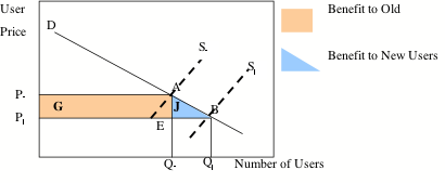
Figure 1: Change in Consumers' Surplus
Consumers’ surplus increases
both for the trips which would
have been taken without the project and for the trips which are stimulated by the project (so-called “induced demand”), as illustrated above in Figure 1. Our analysis is divided into Old and New Trips, the benefits are given in Table 3.
Table 3: Hourly Benefits
TYPE
Old trips
New Trips
Total
Peak
$54,000
$9000
$63,000
Off-peak
$9,000
$500
$9,500
Note: Old Trips: For trips which would have been taken anyway the benefit of the project equals the value of the time saved multiplied by the number of trips. New Trips: The project lowers the cost of a trip and public responds by increasing the number of trips taken. The benefit to new trips is equal to one half of the value of the time saved multiplied by the Fundamentals of Transportation/Evaluation
76
increase in the number of trips. There are 250 weekdays (excluding holidays) each year and four rush hours per weekday. There are 1000 peak hours per year. With 8760 hours per
year, we get 7760 offpeak hours per year. These numbers permit the calculation of annual benefits (shown in Table 4).
Table 4: Annual Travel Time
Benefits
TYPE
Old trips
New Trips
Total
Peak
$54,000,000
$9,000,000
$63,000,000
Off-peak
$69,840,000
$3,880,000
$73,720,000
Total
$123,840,000
$12,880,000
$136,720,000
The safety benefits of the project are the product of the number of lives saved multiplied by the value of life. Typical values of life are on the order of $3,000,000 in US transportation analyses. We need to value life to determine how to trade off between safety investments and other investments. While your life is invaluable to you (that is, I could not pay you enough to allow me to kill you), you don’t act that way when considering chance of death rather than certainty. You take risks that have small probabilities of very bad
consequences. You do not invest all of your resources in reducing risk, and neither does society. If the project is expected to save one life per year, it has a safety benefit of $3,000,000. In a more complete analysis, we would need to include safety benefits from
non-fatal accidents.
The annual benefits of the project are given in Table 5. We assume that this level of benefits continues at a constant rate over the life of the project.
Table 5: Total Annual Benefits
Type of Benefit
Value of Benefits Per Year
Time Saving
$136,720,000
Reduced Risk
$3,000,000
Total
$139,720,000
Costs
Highway costs consist of right-of-way, construction, and maintenance. Right-of-way
includes the cost of the land and buildings that must be acquired prior to construction. It does not consider the opportunity cost of the right-of-way serving a different purpose. Let the cost of right-of-way be $100 million, which must be paid before construction starts. In principle, part of the right-of-way cost can be recouped if the highway is not rebuilt in place (for instance, a new parallel route is constructed and the old highway can be sold for
development). Assume that all of the right-of-way cost is recoverable at the end of the
thirty-year lifetime of the project. The $1 billion construction cost is spread uniformly over the first four-years. Maintenance costs $2 million per year once the highway is completed.
The schedule of benefits and costs for the project is given in Table 6.

Fundamentals of Transportation/Evaluation
77
Table 6: Schedule Of
Benefits And Costs ($
millions)
Time (year)
Benefits
Right-of-way costs Construction costs Maintenance costs
0
0
100
0
0
1-4
0
0
250
0
5-29
139.72
0
0
2
30
139.72
-100
0
2
Conversion to Present Value
The benefits and costs are in constant value dollars. Assume the real interest rate
(excluding inflation) is 2%. The following equations provide the present value of the
streams of benefits and costs.
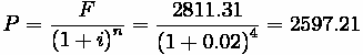
To compute the Present Value of Benefits in Year 5, we apply equation (2) from above.
To convert that Year 5 value to a Year 1 value, we apply equation (1)
The present value of right-of-way costs is computed as today’s right of way cost ($100 M) minus the present value of the recovery of those costs in Year 30, computed with equation (1):
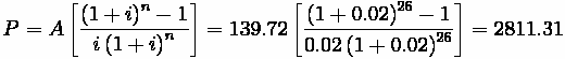
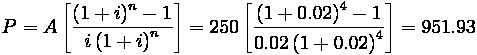
The present value of the construction costs is computed as the stream of $250M outlays
over four years is computed with equation (2):
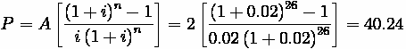
Maintenance Costs are similar to benefits, in that they fall in the same time periods. They are computed the same way, as follows: To compute the Present Value of $2M in
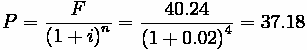
Maintenance Costs in Year 5, we apply equation (2) from above.
To convert that Year 5 value to a Year 1 value, we apply equation (1)
As Table 7 shows, the benefit/cost ratio of 2.5 and the positive net present value of
$1563.31 million indicate that the project is worthwhile under these assumptions (value of time, value of life, discount rate, life of the road). Under a different set of assumptions, (e.g.
a higher discount rate), the outcome may differ.
Table 7: Present Value of Benefits and Costs ($ millions)
Fundamentals of Transportation/Evaluation
78
Present Value
Benefits
2,597.21
Costs
Right-of-Way
44.79
Construction
951.93
Maintenance
37.18
Costs SubTotal
1,033.90
Net Benefit (B-C)
1,563.31
Benefit/Cost Ratio
2.5
Thought Question
Problem
Is money the only thing that matters in Benefit-Cost Analysis? Is "converted" money the only thing that matters? For example, the value of human life in dollars?
Solution
Absolutely not. A lot of benefits and costs can be converted to monetary value, but not all.
For example, you can put a price on human safety, but how can you put a price on, say,
asthetics--something that everyone agrees is beneficial. What else can you think of?
Sample Problems
Key Terms
• Benefit-Cost Analysis
• Profits
• Costs
• Discount Rate
• Present Value
• Future Value
External Exercises
Use the SAND software at the STREET website [3] to learn how to evaluate network performance given a changing network scenario.
End Notes
[1] benefit-cost analysis is sometimes referred to as cost-benefit analysis (CBA)
[2] http://www.sjsu.edu/faculty/watkins/cba.htm
• Aruna, D. Social Cost-Benefit Analysis Madras Institute for Financial Management and
Research, pp. 124, 1980.
• Boardman, A. et al., Cost-Benefit Analysis: Concepts and Practice, Prentice Hall, 2nd Ed, Fundamentals of Transportation/Evaluation
79
• Dorfman, R, “Forty years of Cost-Benefit Analysis: Economic Theory Public Decisions
Selected Essays of Robert Dorfman”, pp. 323, 1997.
• Dupuit, Jules. “On the Measurement of the Utility of Public Works R.H. Babcock (trans.).”