Fundamentals of Transportation by Michael Corbett, Adam Danczyk, et al - HTML preview
Download the book in PDF, ePub, Kindle for a complete version.
Generation/Solution
Problem:
Planners have estimated the following models for the AM Peak Hour
Where:
= Person Trips Originating in Zone
= Person Trips Destined for Zone
= Number of Households in Zone
You are also given the following data
Data
Variable
Dakotopolis
New Fargo
10000
15000
8000
10000
3000
5000
2000
1500
A. What are the number of person trips originating in and destined for each city?
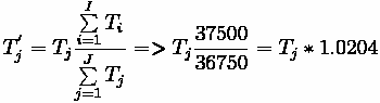
B. Normalize the number of person trips so that the number of person trip origins = the
number of person trip destinations. Assume the model for person trip origins is more
accurate.
Solution:
A. What are the number of person trips originating in and destined for each
city?
Solution to Trip Generation Problem Part A
Households (
Office
Other
Retail
Origins
Destinations
)
Employees (
Employees (
Employees (
)
)
)
Dakotopolis
10000
8000
3000
2000
15000
16000
New Fargo
15000
10000
5000
1500
22500
20750
Total
25000
18000
8000
3000
37500
36750
B. Normalize the number of person trips so that the number of person trip origins = the
number of person trip destinations. Assume the model for person trip origins is more


Fundamentals of Transportation/Trip Generation/Solution
29
accurate.
Use:
Solution to Trip Generation Problem Part B
Origins (
)
Destinations (
)
Adjustment
Normalized
Rounded
Factor
Destinations (
)
Dakotopolis
15000
16000
1.0204
16326.53
16327
New Fargo
22500
20750
1.0204
21173.47
21173
Total
37500
36750
1.0204
37500
37500
Fundamentals of Transportation/
Destination Choice
Everything is related to everything else, but near things are more related than distant things. - Waldo Tobler's 'First Law of Geography’
Trip distribution (or destination choice or zonal interchange analysis), is the second
component (after Trip Generation, but before Mode Choice and Route Choice) in the
traditional four-step transportation forecasting model. This step matches tripmakers’
origins and destinations to develop a “trip table”, a matrix that displays the number of trips going from each origin to each destination. Historically, trip distribution has been the least developed component of the transportation planning model.
Table: Illustrative Trip Table
Origin \ Destination
1
2
3
Z
1
T11
T12
T13
T1Z
2
T21
3
T31
Z
TZ1
TZZ
Where:
= Trips from origin i to destination j. Work trip distribution is the way that travel demand models understand how people take jobs. There are trip distribution models for other (non-work) activities, which follow the same structure.


Fundamentals of Transportation/Destination Choice
30
Fratar Models
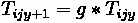
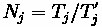
The simplest trip distribution models (Fratar or Growth models) simply extrapolate a base year trip table to the future based on growth,
where:
•
- Trips from to in year
•
- growth factor
Fratar Model takes no account of changing spatial accessibility due to increased supply or changes in travel patterns and congestion.
Gravity Model
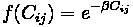
The gravity model illustrates the macroscopic relationships between places (say homes and workplaces). It has long been posited that the interaction between two locations declines with increasing (distance, time, and cost) between them, but is positively associated with the amount of activity at each location (Isard, 1956). In analogy with physics, Reilly (1929) formulated Reilly's law of retail gravitation, and J. Q. Stewart (1948) formulated definitions of demographic gravitation, force, energy, and potential, now called accessibility (Hansen, 1959). The distance decay factor of
has been updated to a more comprehensive
function of generalized cost, which is not necessarily linear - a negative exponential tends to be the preferred form. In analogy with Newton’s law of gravity, a gravity model is often used in transportation planning.
The gravity model has been corroborated many times as a basic underlying aggregate
relationship (Scott 1988, Cervero 1989, Levinson and Kumar 1995). The rate of decline of the interaction (called alternatively, the impedance or friction factor, or the utility or propensity function) has to be empirically measured, and varies by context.
Limiting the usefulness of the gravity model is its aggregate nature. Though policy also operates at an aggregate level, more accurate analyses will retain the most detailed level of information as long as possible. While the gravity model is very successful in explaining the choice of a large number of individuals, the choice of any given individual varies greatly from the predicted value. As applied in an urban travel demand context, the disutilities are primarily time, distance, and cost, although discrete choice models with the application of more expansive utility expressions are sometimes used, as is stratification by income or auto ownership.
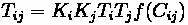
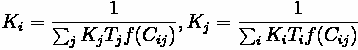
Mathematically, the gravity model often takes the form:
where
•
= Trips between origin and destination
•
= Trips originating at
•
= Trips destined for
•
= travel cost between and
•
= balancing factors solved iteratively.


Fundamentals of Transportation/Destination Choice
31
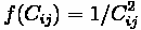
•
= impedance or distance decay factor
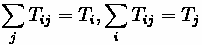
It is doubly constrained so that Trips from to equal number of origins and destinations.
Balancing a matrix
1. Assess Data, you have
,
,
2. Compute
, e.g.
•
•
3. Iterate to Balance Matrix
(a) Multiply Trips from Zone (
) by Trips to Zone (
) by Impedance in Cell
(
) for all
(b) Sum Row Totals
, Sum Column Totals
(c) Multiply Rows by
(d) Sum Row Totals
, Sum Column Totals
(e) Compare
and
,
if within tolerance stop, Otherwise goto (f)
(f) Multiply Columns by
(g) Sum Row Totals
, Sum Column Totals
(h) Compare
and
,
and
if within tolerance stop, Otherwise goto (b)
Issues
Feedback
One of the key drawbacks to the application of many early models was the inability to take account of congested travel time on the road network in determining the probability of
making a trip between two locations. Although Wohl noted as early as 1963 research into
the feedback mechanism or the “interdependencies among assigned or distributed volume,
travel time (or travel ‘resistance’) and route or system capacity”, this work has yet to be widely adopted with rigorous tests of convergence or with a so-called “equilibrium” or
“combined” solution (Boyce et al. 1994). Haney (1972) suggests internal assumptions about travel time used to develop demand should be consistent with the output travel times of the route assignment of that demand. While small methodological inconsistencies are
necessarily a problem for estimating base year conditions, forecasting becomes even more tenuous without an understanding of the feedback between supply and demand. Initially
heuristic methods were developed by Irwin and Von Cube (as quoted in Florian et al. (1975)
) and others, and later formal mathematical programming techniques were established by
Evans (1976).
Feedback and time budgets
A key point in analyzing feedback is the finding in earlier research by Levinson and Kumar (1994) that commuting times have remained stable over the past thirty years in the
Washington Metropolitan Region, despite significant changes in household income, land
use pattern, family structure, and labor force participation. Similar results have been found in the Twin Cities by Barnes and Davis (2000).


Fundamentals of Transportation/Destination Choice
32
The stability of travel times and distribution curves over the past three decades gives a good basis for the application of aggregate trip distribution models for relatively long term forecasting. This is not to suggest that there exists a constant travel time budget.
In terms of time budgets:
• 1440 Minutes in a Day
• Time Spent Traveling: ~ 100 minutes + or -
• Time Spent Traveling Home to Work: 20 - 30 minutes + or -
Research has found that auto commuting times have remained largely stable over the past
forty years, despite significant changes in transportation networks, congestion, household income, land use pattern, family structure, and labor force participation. The stability of travel times and distribution curves gives a good basis for the application of trip
distribution models for relatively long term forecasting.
Examples
Example 1: Solving for impedance
Problem:
You are given the travel times between zones, compute the impedance matrix
,
assuming
.
Travel Time OD Matrix (
Origin Zone
Destination Zone 1
Destination Zone 2
1
2
5
2
5
2
Compute impedances (
)
Solution:
Impedance Matrix (
Origin Zone
Destination Zone 1
Destination Zone 2
1
2


Fundamentals of Transportation/Destination Choice
33
Example 2: Balancing a Matrix Using Gravity Model
Problem:
You are given the travel times between zones, trips originating at each zone (zone1 =15, zone 2=15) trips destined for each zone (zone 1=10, zone 2 = 20) and asked to use the
classic gravity model
Travel Time OD Matrix (
Origin Zone
Destination Zone 1
Destination Zone 2
1
2
5
2
5
2
Solution:
(a) Compute impedances (
)
Impedance Matrix (
Origin Zone
Destination Zone 1
Destination Zone 2
1
0.25
0.04
2
0.04
0.25
(b) Find the trip table
Balancing Iteration 0 (Set-up)
Origin Zone
Trips Originating
Destination Zone 1
Destination Zone 2
Trips Destined
10
20
1
15
0.25
0.04
2
15
0.04
0.25
Balancing Iteration 1 (
Origin Zone
Trips
Destination Zone 1 Destination Zone 2 Row Total
Normalizing
Originating
Factor
Trips Destined
10
20
1
15
37.50
12
49.50
0.303
2
15
6
75
81
0.185
Column Total
43.50
87


Fundamentals of Transportation/Destination Choice
34
Balancing Iteration 2 (
Origin Zone
Trips
Destination Zone
Destination Zone
Row Total
Normalizing
Originating
1
2
Factor
Trips Destined
10
20
1
15
11.36
3.64
15.00
1.00
2
15
1.11
13.89
15.00
1.00
Column Total
12.47
17.53
Normalizing
0.802
1.141
Factor
Balancing Iteration 3 (
Origin Zone
Trips
Destination Zone
Destination Zone
Row
Normalizing
Originating
1
2
Total
Factor
Trips Destined
10
20
1
15
9.11
4.15
13.26
1.13
2
15
0.89
15.85
16.74
0.90
Column Total
10.00
20.00
Normalizing
1.00
1.00
Factor =
Balancing Iteration 4 (
Origin Zone
Trips
Destination Zone
Destination Zone
Row
Normalizing
Originating
1
2