Understanding Galaxy Formation and Evolution by Vladimir Avila-Reese - HTML preview
Download the book in PDF, ePub, Kindle for a complete version.
12 The mathematical solution gives that the spherical perturbed region collapses
into a point (a black hole) after reaching its maximum expansion. However, real
perturbations are lumpy and the particle orbits are not perfectly radial. In this
situation, during the collapse the structure comes to a dynamical equilibrium un-
der the influence of large scale gravitational potential gradients, a process named
by the oxymoron “violent relaxation” (see e.g. [14]); this is a typical collective phenomenon. The end result is a system that satisfies the virial theorem: for
a self–gravitating system this means that the internal kinetic energy is half the
(negative) gravitational potential energy. Gravity is supported by the velocity dis-
persion of particles or lumps. The collapse factor is roughly 1/2, i.e. the typical
virial radius Rv of the collapsed structure is ≈ 0.5 the radius of the perturbation
at its maximum expansion.


Understanding Galaxy Formation and Evolution
27
where a good approximation for g(z) is [23]:
5
−1
4
Ω
Ω
g(z) ≃
Ω
M
Λ
7
1 +
,
(13)
2
M − ΩΛ +
1 + 2
70
and where ΩM = ΩM,0(1 + z)3/E2(z), ΩΛ = ΩΛ/E2(z), with E2(z) = ΩΛ +
ΩM,0 (1 + z)3. For the Einstein–de Sitter model, D(z) = (1 + z). We need
now to connect the top–hat sphere results to a perturbation of mass M . The
processed perturbation field, fixed at the present epoch, is characterized by the
mass variance σM and we may assume that δ0 = νσM , where δ0 is δ linearly
extrapolated to z = 0, and ν is the peak height. For average perturbations, ν =
1, while for rare, high–density perturbations, from which the first structures
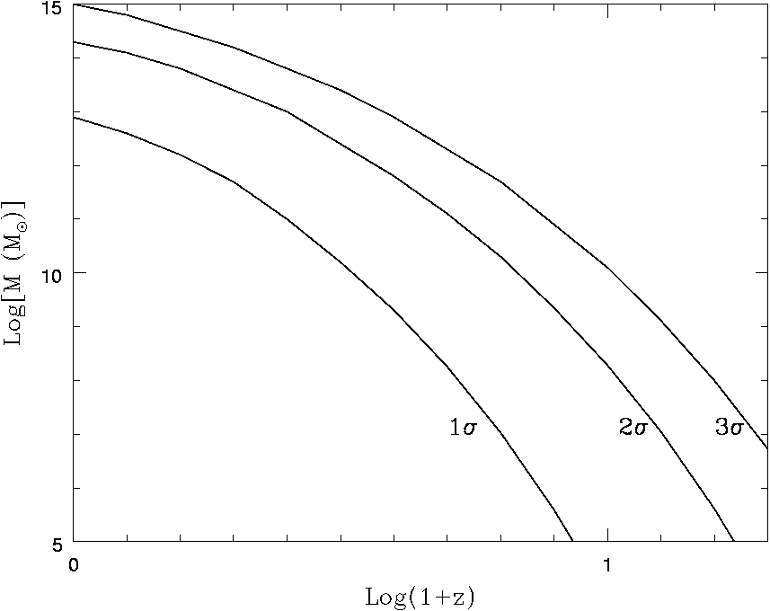
arose, ν >> 1. By introducing δ0 = νσM into eq. (11) one may infer zcol for a given mass. Fig. 7 shows the typical zcol of 1σ, 2σ, and 3σ halos. The collapse of galaxy–sized 1σ halos occurs within a relatively small range of
redshifts. This is a direct consequence of the “flattening” suffered by σM
during radiation–dominated era due to stangexpansion (see §3.2). Therefore,
in a ΛCDM Universe it is not expected to observe a significant population of
galaxies at z > 5.
∼
Fig. 7. Collapse redshifts of spherical top–hat 1σ, 2σ and 3σ perturbations in a
ΛCDM cosmology with σ8 = 0.9. Note that galaxy–sized (M ∼ 108 − 1013M⊙)
1σ halos collapse in a redshift range, from z ∼ 3.5 to z = 0, respectively; the
corresponding ages are from ∼ 1.9 to 13.8 Gyr, respectively.
The problem of cosmological gravitational clustering is very complex due
to non–linearity, lack of symmetry and large dynamical range. Analytical
and semi–analytical approaches provide illuminating results but numerical
N–body simulations are necessary to tackle all the aspects of this problem. In
the last 20 years, the “industry” of numerical simulations had an impressive
development. The first cosmological simulations in the middle 80s used a few
104 particles (e.g., [36]). The currently largest simulation (called the Mille-28
Vladimir Avila-Reese
nium simulation [111]) uses ∼ 1010 particles! A main effort is done to reach larger and larger dynamic ranges in order to simulate encompassing volumes
large enough to contain representative populations of all kinds of halos (low
mass and massive ones, in low– and high–density environments, high–peak
rare halos), yet resolving the inner structure of individual halos.
Halo mass function
The CDM halo mass function (comoving number density of halos of different
masses at a given epoch z, n(M, z)) obtained in the N–body simulations is
consistent with the P-S function in general, which is amazing given the ap-
proximate character of the P-S analysis. However, in more detail, the results
of large N–body simulations are better fitted by modified P-S analytical func-
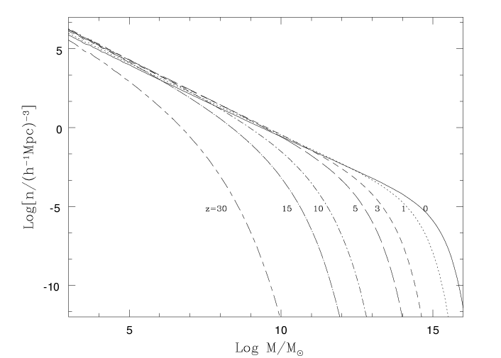
tions, as the one derived in [103] and showed in Fig. 8. Using the Millennium simulation, the halo mass function has been accurately measured in the range
that is well sampled by this run (z ≤ 12, M ≥ 1.7 × 10¹⁰M⊙h−1). The mass
function is described by a power law at low masses and an exponential cut–off
at larger masses. The “cut-off”, most typical mass, increases with time and
is related to the hierarchical evolution of the 1σ halos shown in Fig. 7. The halo mass function is the starting point for modeling the luminosity function of galaxies. From Fig. 8 we see that the evolution of the abundances of massive halos is much more pronounced than the evolution of less massive
halos. This is why observational studies of abundance of massive galaxies or
cluster of galaxies at high redshifts provide a sharp test to theories of cosmic
structure formation. The abundance of massive rare halos at high redshifts
are for example a strong function of the fluctuation field primordial statistics
(Gaussianity or non-Gaussianity).
Subhalos. An important result of N–body simulations is the existence of sub-
halos, i.e. halos inside the virial radius of larger halos, which survived as
self–bound entities the gravitational collapse of the higher level of the hier-
archy. Of course, subhalos suffer strong mass loss due to tidal stripping, but
this is probably not relevant for the luminous galaxies formed in the inner-
most regions of (sub)halos. This is why in the case of subhalos, the maximum
circular velocity Vm (attained at radii much smaller than the virial radius) is
used instead of the virial mass. The Vm distribution of subhalos inside cluster–
sized and galaxy–sized halos is similar [83]. This distribution agrees with the distribution of galaxies seen in clusters, but for galaxy–sized halos the number
of subhalos overwhelms by 1–2 orders of magnitude the observed number of
satellite galaxies around galaxies like Milky Way and Andromeda [70, 83].
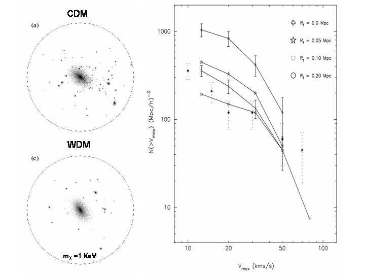
Fig. 9 (right side) shows the subhalo cumulative Vm−distribution for a CDM Milky Way–like halo compared to the observed satellite Vm−distribution.
In this Fig. are also shown the Vm−distributions obtained for the same Milky–
Way halo but using the power spectrum of three WDM models with particle
masses mX ≈ 0.6, 1, and 1.7 KeV. The smaller mX, the larger is the free–
streaming (filtering) scale, Rf , and the more substructure is washed out (see
Understanding Galaxy Formation and Evolution
29
Fig. 8. Evolution of the comoving number density of collapsed halos (P–S mass
function) according to the ellipsoidal modification by [103]. Note that the “cut–off”
mass grows with time. Most of the mass fraction in collapsed halos at a given epoch
are contained in halos with masses around the “cut–off” mass.
§3.2). In the left side of Fig. 9 is shown the DM distribution inside the Milky–
Way halo simulated by using a CDM power spectrum (top) and a WDM
power spectrum with mX ≈ 1KeV (sterile neutrino, bottom). For a student it
should be exciting to see with her(his) own eyes this tight connection between
micro– and macro–cosmos: the mass of the elemental particle determines the
structure and substructure properties of galaxy halos!
Halo density profiles
High–resolution N–body simulations [87] and semi–analytical techniques (e.g.,
[3]) allowed to answer the following questions: How is the inner mass distribution in CDM halos? Does this distribution depend on mass? How universal
is it? The two–parameter density profile established in [87] (the Navarro-Frenk-White, NFW profile) departs from a single power law, and it was
proposed to be universal and not depending on mass. In fact the slope
β(r) ≡ −dlogρ(r)/dlogr of the NFW profile changes from −1 in the cen-
ter to −3 in the periphery. The two parameters, a normalization factor, ρs
and a shape factor, rs, were found to be related in a such a way that the profile
depends only on one shape parameter that could be expressed as the concen-
tration, cNF W ≡ rs/Rv. The more massive the halo, the less concentrated on
the average. For the ΛCDM model, c ≈ 20−5 for M ∼ 2×10⁸−2×10¹⁵M⊙h−1,
respectively [42]. However, for a given M , the scatter of cNF W is large (≈ 30 − 40%), and it is related to the halo formation history [3, 21, 125] (see
30
Vladimir Avila-Reese
Fig. 9. Dark matter distribution in a sphere of 400Mpch−1 of a simulated Galaxy–
sized halo with CDM (a) and WDM (mX = 1KeV, b). The substructure in the
latter case is significantly erased. Right panel shows the cumulative maximum Vc
distribution for both cases (open crosses and squares, respectively) as well as for an
average of observations of satellite galaxies in our Galaxy and in Andromeda (dotted
error bars). Adapted from [31] .
below). A significant fraction of halos depart from the NFW profile. These
are typically not relaxed or disturbed by companions or external tidal forces.
Is there a “cusp” crisis? More recently, it was found that the inner density
profile of halos can be steeper than β = −1 (e.g. [84]). However, it was shown that in the limit of resolution, β never is as steep a −1.5 [88]. The inner structure of CDM halos can be tested in principle with observations of (i) the
inner rotation curves of DM dominated galaxies (Irr dwarf and LSB galaxies;
the inner velocity dispersion of dSph galaxies is also being used as a test
), and (ii) strong gravitational lensing and hot gas distribution in the inner
regions of clusters of galaxies. Observations suggest that the DM distribution
in dwarf and LSB galaxies has a roughly constant density core, in contrast
to the cuspy cores of CDM halos (the literature on this subject is extensive;
see for recent results [37, 50, 107, 128] and more references therein). If the observational studies confirm that halos have constant–density cores, then
either astrophysical mechanisms able to expand the halo cores should work
efficiently or the ΛCDM scenario should be modified. In the latter case, one of

Understanding Galaxy Formation and Evolution
31
the possibilities is to introduce weakly self–interacting DM particles. For small
cross sections, the interaction is effective only in the more dense inner regions
of galaxies, where heat inflow may expand the core. However, the gravo–
thermal catastrophe can also be triggered. In [32] it was shown that in order to avoid the gravo–thermal instability and to produce shallow cores with densities
approximately constant for all masses, as suggested by observations, the DM
cross section per unit of particle mass should be σDM /mX = 0.5 − 1.0v−1
100
cm2/gr, where v100 is the relative velocity of the colliding particles in unities
of 100 km/s; v100 is close to the halo maximum circular velocity, Vm.
The DM mass distribution was inferred from the rotation curves of dwarf
and LSB galaxies under the assumptions of circular motion, halo spherical
symmetry, the lack of asymmetrical drift, etc. In recent studies it was discussed
that these assumptions work typically in the sense of lowering the observed
inner rotation velocity [59, 100, 118]. For example, in [118] it is demonstrated that non-circular motions (due to a bar) combined with gas pressure support
and projection effects systematically underestimate by up to 50% the rotation
velocity of cold gas in the central 1 kpc region of their simulated dwarf galaxies,
creating the illusion of a constant density core.
Mass–velocity relation. In a very simplistic analysis, it is easy to find that
M ∝ V 3
c
if the average halo density ρh does not depend on mass. On one
hand, Vc ∝ (GM/R)1/2, and on the other hand, ρh ∝ M/R3, so that Vc ∝
M 1/3ρ1/6. Therefore, for ρ
h
h =const, M ∝ V 3
c . We have seen in §3.2 that
the CDM perturbations at galaxy scales have similar amplitudes (actually
σM ∝ lnM) due to the stangexpansion effect in the radiation–dominated era.
This implies that galaxy–sized perturbations collapse within a small range
of epochs attaining more or less similar average densities. The CDM halos
actually have a mass distribution that translates into a circular velocity profile
Vc(r). The maximum of this profile, Vm, is typically the circular velocity that
characterizes a given halo of virial mass M . Numerical and semi–numerical
results show that (ΛCDM model):
3.2
M ≈ 5.2 × 10⁴
Vm
M
kms−1
⊙h−1,
(14)
Assuming that the disk infrared luminosity LIR ∝ M, and that the disk
maximum rotation velocity Vrot,m ∝ Vm, one obtains that LIR ∝ V 3.2
rot,m,
amazingly similar to the observed infrared Tully–Fisher relation [116], one of the most robust and intriguingly correlations in the galaxy world! I conclude
that this relation is a clear imprint of the CDM power spectrum of fluctuations.
Mass assembling histories
One of the key concepts of the hierarchical clustering scenario is that cos-
mic structures form by a process of continuous mass aggregation, opposite to
the monolithic collapse scenario. The mass assembly of CDM halos is charac-
terized by the mass aggregation history (MAH), which can alternate smooth
32
Vladimir Avila-Reese
mass accretion with violent major mergers. The MAH can be calculated by using semi–analytical approaches based on extensions of the P-S formalism.
The main idea lies in the estimate of the conditional probability that given a
collapsed region of mass M0 at z0, a region of mass M1 embedded within the
volume containing M0, had collapsed at an earlier epoch z1. This probability
is calculated based on the excursion set formalism starting from a Gaussian
density field characterized by an evolving mass variance σM [17, 73]. By using the conditional probability and random trials at each temporal step, the
“backward” MAHs corresponding to a fixed mass M0 (defined for instance at
z = 0) can be traced. The MAHs of isolated halos by definition decrease to-
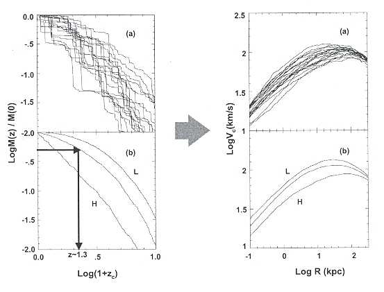
ward the past, following different tracks (Fig. 10), sometimes with abrupt big jumps that can be identified as major mergers in the halo assembly history.
Fig. 10. Upper panels (a). A score of random halo MAHs for a present–day virial mass of 3.5 × 10¹¹M⊙ and the corresponding circular velocity profiles of the virialized halos. Lower panels (b). The average MAH and two extreme deviations from
104 random MAHs for the same mass as in (a), and the corresponding halo cir-
cular velocity profiles. The MAHs are diverse for a given mass and the Vc (mass)
distribution of the halos depend on the MAH. Adapted from [45] .
Understanding Galaxy Formation and Evolution
33
To characterize typical behaviors of the halo MAHs, one may calculate the
average MAH for a given virial mass M0, for a given “population” of halos
selected by its environment, etc. In the left panels of Fig. 10 are shown 20
individual MAHs randomly selected from 104 trials for M0 = 3.5 × 10¹¹M⊙ in
a ΛCDM cosmology [45]. In the bottom panel are plotted the average MAH
from these 104 trials as well as two extreme deviations from the average. The
average MAHs depend on mass: more massive halos have a more extended
average MAH, i.e. they aggregate a given fraction of M0 latter than less mas-
sive halos. It is a convention to define the typical halo formation redshift, zf ,
when half of the current halo mass M0 has been aggregated. For instance, for
the ΛCDM cosmology the average MAHs show that zf ≈ 2.2, 1.2 and 0.7 for
M0 = 1010M⊙, 1012M⊙ and 1014M⊙, respectively. A more physical definition
of halo formation time is when the halo maximum circular velocity Vm attains
its maximum value. After this epoch, the mass can continue growing, but the
inner gravitational potential of the system is already set.
Right panels of Fig. 10 show the present–day halo circular velocity profiles, Vc(r), corresponding to the MAHs plotted in the left panels. The average
Vc(r) is well described by the NFW profile. There is a direct relation between
the MAH and the halo structure as described by Vc(r) or the concentration
parameter. The later the MAH, the more extended is Vc(r) and the less con-
centrated is the halo [3, 125]. Using high–resolution simulations some authors have shown that the halo MAH presents two regimes: an early phase of fast
mass aggregation (mainly by major mergers) and a late phase of slow aggre-
gation (mainly by smooth mass accretion) [133, 75]. The potential well of a present–day halo is set mainly at the end of the fast, major–merging driven,
growth phase.
From the MAHs we may infer: (i) the mass aggregation rate evolution of
halos (halo mass aggregated per unit of time at different z′s), and (ii) the ma-
jor merging rates of halos (number of major mergers per unit of time per halo
at different z′s). These quantities should be closely related to the star forma-
tion rates of the galaxies formed within the halos as well as to the merging of
luminous galaxies and pair galaxy statistics. By using the ΛCDM model, sev-
eral studies showed that most of the mass of the present–day halos has been
aggregated by accretion rather than major mergers (e.g., [85]). Major merging was more frequent in the past [55], and it is important for understanding the formation of massive galaxy spheroids and the phenomena related to this
process like QSOs, supermassive black hole growth, obscured star formation
bursts, etc. Both the mass aggregation rate and major merging rate histories
depend strongly on environment: the denser the environment, the higher is
the merging rate in the past. However, in the dense environments (group and
clusters) form typically structures more massive than in the less dense regions
(field and voids). Once a large structure virializes, the smaller, galaxy–sized
halos become subhalos with high velocity dispersions: the mass growth of the
subhalos is truncated, or even reversed due to tidal stripping, and the merging
probability strongly decreases. Halo assembling (and therefore, galaxy assem-

34
Vladimir Avila-Reese
bling) definitively depends on environment. Overall, by integrating the MAHs
of the whole galaxy–sized ΛCDM halo population in a given volume, the gen-
eral result is that the peak in halo assembling activity was at z ≈ 1 − 2. After
these redshifts, the global mass aggregation rate strongly decreases (e.g., [121].
To illustrate the driving role of DM processes in galaxy evolution, I men-
tion briefly here two concrete examples:
1). Distributions of present–day specific mass aggregation rate, ( ˙
M /M )0 ,
and halo lookback formation time, T1/2 . For a ΛCDM model, these distributions are bimodal, in particular the former. We have found that roughly
40% of halos (masses larger than ≈ 1011M⊙h−1) have ( ˙
M /M )0 ≤ 0; they
are basically subhalos. The remaining 60% present a broad distribution of
( ˙
M /M )0 > 0 peaked at ≈ 0.04Gyr−1. Moreover, this bimodality strongly
changes with large–scale environment: the denser is the environment the,
higher is the fraction of halos with ( ˙
M /M )0 ≤ 0. It is interesting enough
that similar fractions and dependences on environment are found for the spe-
cific star formation rates of galaxies in large statistical surveys (§§2.3); the
situation is similar when confronting the distributions of T1/2 and observed
colors. Therefore, it seems that the the main driver of the observed bimodal-
ities in z = 0 specific star formation rate and color of galaxies is the nature of the CDM halo mass aggregation process. Astrophysical processes of course
are important but the main body of the bimodalities can be explained just at
the level of DM processes.
2. Major merging rates. The observational inference of galaxy major merg-
ing rates is not an easy task. The two commonly used methods are based on
the statistics of galaxy pairs (pre–mergers) and in the morphological distor-
tions of ellipticals (post–mergers). The results show that the merging rate
increases as (1 + z)x, with x ∼ 0 − 4. The predicted major merging rates in
the ΛCDM scenario agree roughly with those inferred from statistics of galaxy
pairs. From the fraction of normal galaxies in close companions (with sepa-
rations less than 50 kpch−1) inferred from observations at z = 0 and z = 0.3
[91], and assuming an average merging time of ∼ 1 Gyr for these separations, we estimate that the major merging rate at the present epoch is ∼ 0.01 Gyr−1
for halos in the range of 0.1 − 2.0 1012M⊙, while at z = 0.3 the rate increased
to ∼ 0.018 Gyr−1. These values are only slightly lower than predictions for
the ΛCDM model.
Angular momentum
The origin of the angular momentum (AM) is a key ingredient in theories of
galaxy formation. Two mechanisms of AM acquirement were proposed for the
CDM halos (e.g., [93, 22, 78]): 1. tidal torques of the surrounding shear field when the perturbation is still in the linear regime, and 2. transfer of orbital AM
to internal AM in major and minor mergers of collapsed halos. The angular
momentum of DM halos is parametrized in terms of the dimensionless spin
√
parameter λ ≡ J E/(GM5/2, where J is the modulus of the total angular


Understanding Galaxy Formation and Evolution
35
momentum and E is the total (kinetic plus potential). It is easy to show that λ
can be interpreted as the level of rotational support of a gravitational system,
λ = ω/ωsup, where ω is the angular velocity of the system and ωsup is the
angular velocity needed for the system to be rotationally supported against
gravity (see [90]).
For disk and elliptical galaxies, λ ∼ 0.4−0.8 and ∼ 0.01−0.05, respectively.
Cosmol