Kinematics fundamentals by Sunil Singh - HTML preview
Download the book in PDF, ePub for a complete version.
motion, when paths followed by the particles, composing the body are parallel to each other (See
Figure). As we are concerned with the geometry of the path of motion in kinematics, it is,
therefore, reasonable to treat real bodies as “point like” mass for description of translational
motion.
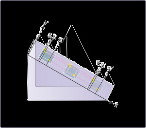
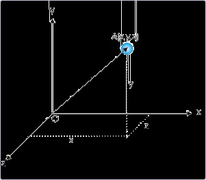
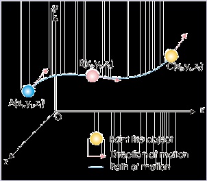
Figure 1.20. Translational motion
Particles follow parallel paths
We conceptualize a particle in order to facilitate the geometric description of motion. A particle is
considered to be dimensionless, but having a mass. This hypothetical construct provides the basis
for the logical correspondence of point with the position occupied by a particle.
Without any loss of purpose, we can designate motion to begin at A or A’ or A’’ corresponding to
final positions B or B’ or B’’ respectively as shown in the figure above.
For the reasons as outlined above, we shall freely use the terms “body” or “object” or “particle” in
one and the same way as far as description of translational motion is concerned. Here, pure
translation conveys the meaning that the object is under motion without rotation, like sliding of a
block on a smooth inclined plane.
Position
Definition: Position
The position of a particle is a point in the defined volumetric space of the coordinate system.
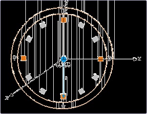
Figure 1.21. Position of a point object
Position of a point is specified by three coordinate values
The position of a point like object, in three dimensional coordinate space, is defined by three
values of coordinates i.e. x, y and z in Cartesian coordinate system as shown in the figure above.
It is evident that the relative position of a point with respect to a fixed point such as the origin of
the system “O” has directional property. The position of the object, for example, can lie either to
the left or to the right of the origin or at a certain angle from the positive x - direction. As such the
position of an object is associated with directional attribute with respect to a frame of reference
(coordinate system).
Example 1.2. Coordinates
Problem : The length of the second’s hand of a round wall clock is ‘r’ meters. Specify the
coordinates of the tip of the second’s hand corresponding to the markings 3,6,9 and 12
(Consider the center of the clock as the origin of the coordinate system.).
Figure 1.22. Coordinates of the tip of the second’s hand
The origin coincides with the center
Solution : The coordinates of the tip of the second’s hand is given by the coordinates :
3 : r, 0, 0
6 : 0, -r, 0
9 : -r, 0, 0
12 : 0, r, 0
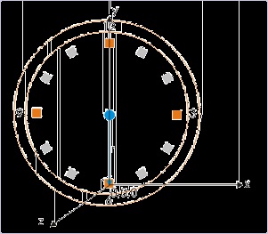
What would be the coordinates of the markings 3,6,9 and 12 in the earlier example, if the origin
coincides with the marking 6 on the clock ?
Figure 1.22. Coordinates of the tip of the second’s hand
Origin coincides with the marking 6 O’ clock
The coordinates of the tip of the second’s hand is given by the coordinates :
3 : r, r, 0
6 : 0, 0, 0
9 : -r, r, 0
12 : 0, 2r, 0
The above exercises point to an interesting feature of the frame of reference: that the specification
of position of the object (values of coordinates) depends on the choice of origin of the given frame
of reference. We have already seen that description of motion depends on the state of observer i.e.
the attached system of reference. This additional dependence on the choice of origin of the
reference would have further complicated the issue, but for the linear distance between any two
points in a given system of reference, is found to be independent of the choice of the origin. For
example, the linear distance between the markings 6 and 12 is ‘2r’, irrespective of the choice of
the origin.
Plotting motion
Position of a point in the volumetric space is a three dimensional description. A plot showing
positions of an object during a motion is an actual description of the motion in so far as the curve
shows the path of the motion and its length gives the distance covered. A typical three
dimensional motion is depicted as in the figure below :
Figure 1.23. Motion in three dimension
The plot is the path followed by the object during motion.
In the figure, the point like object is deliberately shown not as a point, but with finite dimensions.
This has been done in order to emphasize that an object of finite dimensions can be treated as
point when the motion is purely translational.
The three dimensional description of positions of an object during motion is reduced to be two or
one dimensional description for the planar and linear motions respectively. In two or one
dimensional motion, the remaining coordinates are constant. In all cases, however, the plot of the
positions is meaningful in following two respects :
The length of the curve (i.e. plot) is equal to the distance.
A tangent in forward direction at a point on the curve gives the direction of motion at that point
Description of motion
Position is the basic element used to describe motion. Scalar properties of motion like distance
and speed are expressed in terms of position as a function of time. As the time passes, the
positions of the motion follow a path, known as the trajectory of the motion. It must be
emphasized here that the path of motion (trajectory) is unique to a frame of reference and so is the
description of the motion.
To illustrate the point, let us consider that a person is traveling on a train, which is moving with
the velocity v along a straight track. At a particular moment, the person releases a small pebble.
The pebble drops to the ground along the vertical direction as seen by the person.
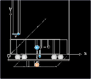
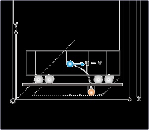
Figure 1.24. Trajectory as seen by the passenger
Trajectory is a straight line.
The same incident, however, is seen by an observer on the ground as if the pebble followed a
parabolic path (See Figure blow). It emerges then that the path or the trajectory of the motion is
also a relative attribute, like other attributes of the motion (speed and velocity). The coordinate
system of the passenger in the train is moving with the velocity of train ( v) with respect to the
earth and the path of the pebble is a straight line. For the person on the ground, however, the
coordinate system is stationary with respect to earth. In this frame, the pebble has a horizontal
velocity, which results in a parabolic trajectory.
Figure 1.25. Trajectory as seen by the person on ground
Trajectory is a parabolic curve.
Without overemphasizing, we must acknowledge that the concept of path or trajectory is
essentially specific to the frame of reference or the coordinate system attached to it. Interestingly,
we must be aware that this particular observation happens to be the starting point for the
development of special theory of relativity by Einstein (see his original transcript on the subject
of relativity).
Position – time plot
The position in three dimensional motion involves specification in terms of three coordinates.
This requirement poses a serious problem, when we want to investigate positions of the object
with respect to time. In order to draw such a graph, we would need three axes for describing
position and one axis for plotting time. This means that a position – time plot for a three
dimensional motion would need four (4) axes !
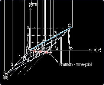
A two dimensional position – time plot, however, is a possibility, but its drawing is highly
complicated for representation on a two dimensional paper or screen. A simple example
consisting of a linear motion in the x-y plane is plotted against time on z – axis (See Figure).
Figure 1.26. Two dimensional position – time plot
As a matter of fact, it is only the one dimensional motion, whose position – time plot can be
plotted conveniently on a plane. In one dimensional motion, the point object can either be to the
left or to the right of the origin in the direction of reference line. Thus, drawing position against
time is a straight forward exercise as it involves plotting positions with appropriate sign.
Example 1.3. Coordinates
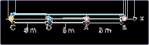
Problem : A ball moves along a straight line from O to A to B to C to O along x-axis as shown
in the figure. The ball covers each of the distance of 5 m in one second. Plot the position –
time graph.
Figure 1.27. Motion along a straight line
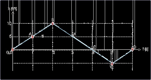
Solution : The coordinates of the ball are 0,5,10, -5 and 0 at points O, A, B, C and O (on
return) respectively. The position – time plot of the motion is as given below :
Figure 1.28. Position – time plot in one dimension
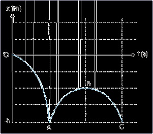
A ball falling from a height ‘h’ strikes a hard horizontal surface with increasing speed. On each
rebound, the height reached by the ball is half of the height it fell from. Draw position – time plot
for the motion covering two consecutive strikes, emphasizing the nature of curve (ignore actual
calculation).
Now, as the ball falls towards the surface, it covers path at a quicker pace. As such, the position
changes more rapidly as the ball approaches the surface. The curve (i.e. plot) is, therefore, steeper
towards the surface. On the return upward journey, the ball covers lesser distance as it reaches the
maximum height. Hence, the position – time curve (i.e. plot) is flatter towards the point of
maximum height.
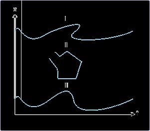
Figure 1.28. Position – time plot in one dimension
The figure below shows three position – time plots of a motion of a particle along x-axis. Giving
reasons, identify the valid plot(s) among them. For the valid plot(s), determine following :
Figure 1.28. Position – time plots in one dimension
1. How many times the particle has come to rest?
2. Does the particle reverse its direction during motion?
Validity of plots : In the portion of plot I, we can draw a vertical line that intersects the curve at
three points. It means that the particle is present at three positions simultaneously, which is not
possible. Plot II is also not valid for the same reason. Besides, it consists of a vertical portion,
which would mean presence of the particle at infinite numbers of positions at the same instant.
Plot III, on the other hand, is free from these anomalies and is the only valid curve representing
motion of a particle along x – axis (See Figure).
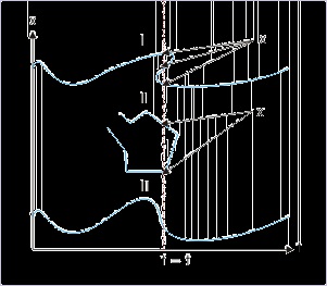
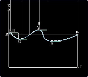
Figure 1.28. Valid position – time plot in one dimension
A particle can not be present at more than one position at a given instant.
When the particle comes to rest, there is no change in the value of “x”. This, in turn, means that
tangent to the curve at points of rest is parallel to x-axis. By inspection, we find that tangent to the
curve is parallel to x-axis at four points (B,C,D and E) on the curve shown in the figure below.
Hence, the particle comes to rest four times during the motion.
Figure 1.28. Positions of rest
At rest, the tangent to the path is parallel to time axis.
1.5. Vectors*
A number of key fundamental physical concepts relate to quantities, which display directional


property. Scalar algebra is not suited to deal with such quantities. The mathematical construct
called vector is designed to represent quantities with directional property. A vector, as we shall
see, encapsulates the idea of “direction” together with “magnitude”.
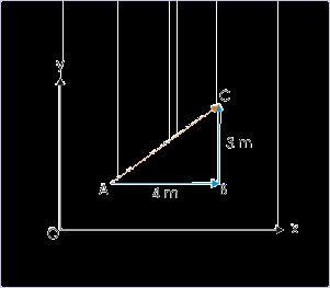
In order to elucidate directional aspect of a vector, let us consider a simple example of the motion
of a person from point A to point B and from point B to point C, covering a distance of 4 and 3
meters respectively as shown in the Figure . Evidently, AC represents the linear distance between the initial and the final positions. This linear distance, however, is not equal to the sum of the
linear distances of individual motion represented by segments AB and BC ( 4 + 3 = 7 m) i.e.
Figure 1.29. Displacement
Scalar inequality
However, we need to express the end result of the movement appropriately as the sum of two
individual movements. The inequality of the scalar equation as above is basically due to the fact
that the motion represented by these two segments also possess directional attributes; the first
segment is directed along the positive x – axis, where as the second segment of motion is directed
along the positive y –axis. Combining their magnitudes is not sufficient as the two motions are
perpendicular to each other. We require a mechanism to combine directions as well.
The solution of the problem lies in treating individual distance with a new term "displacement" –
a vector quantity, which is equal to “linear distance plus direction”. Such a conceptualization of a
directional quantity allows us to express the final displacement as the sum of two individual
displacements in vector form :
The magnitude of displacement is obtained by applying Pythagoras theorem :


It is clear from the example above that vector construct is actually devised in a manner so that
physical reality having directional property is appropriately described. This "fit to requirement"
aspect of vector construct for physical phenomena having direction is core consideration in
defining vectors and laying down rules for vector operation.
A classical example, illustrating the “fit to requirement” aspect of vector, is the product of two
vectors. A product, in general, should evaluate in one manner to yield one value. However, there
are natural quantities, which are product of two vectors, but evaluate to either scalar (example :
work) or vector (example : torque) quantities. Thus, we need to define the product of vectors in
two ways : one that yields scalar value and the other that yields vector value. For this reason
product of two vectors is either defined as dot product to give a scalar value or defined as cross
product to give vector value. This scheme enables us to appropriately handle the situations as the
case may be.
Mathematical concept of vector is basically secular in nature and general in application. This
means that mathematical treatment of vectors is without reference to any specific physical
quantity or phenomena. In other words, we can employ vector and its methods to all quantities,
which possess directional attribute, in a uniform and consistent manner. For example two vectors
would be added in accordance with vector addition rule irrespective of whether vectors involved
represent displacement, force, torque or some other vector quantities.
The moot point of discussion here is that vector has been devised to suit the requirement of
natural process and not the other way around that natural process suits vector construct as defined
in vector mathematics.
What is a vector?
Definition: Vector
Vector is a physical quantity, which has both magnitude and direction.
A vector is represented graphically by an arrow drawn on a scale as shown Figure i. In order to process vectors using graphical methods, we need to draw all vectors on the same scale. The arrow
head point in the direction of the vector.
A vector is notionally represented in a characteristic style. It is denoted as bold face type like “ a ”
as shown Figure (i) or with a small arrow over the symbol like “
” or with a small bar as in “
”. The magnitude of a vector quantity is referred by simple identifier like “a” or as the absolute
value of the vector as “ | a | ” .
Two vectors of equal magnitude and direction are equal vectors ( Figure (ii) ). As such, a vector can be laterally shifted as long as its direction remains same ( Figure (ii) ). Also, vectors can be
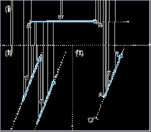
shifted along its line of application represented by dotted line ( Figure (iii) ). The flexibility by virtue of shifting vector allows a great deal of ease in determining vector’s interaction with other
scalar or vector quantities.
Figure 1.30. Vectors
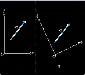
It should be noted that graphical representation of vector is independent of the origin or axes of
coordinate system except for few vectors like position vector (called localized vector), which is
tied to the origin or a reference point by definition. With the exception of localized vector, a
change in origin or orientation of axes or both does not affect vectors and vector operations like
addition or multiplication (see figure below).
Figure 1.31. Vectors
The vector is not affected, when the coordinate is rotated or displaced as shown in the figure
above. Both the orientation and positioning of origin i.e reference point do not alter the vector
representation. It remains what it is. This feature of vector operation is an added value as the study
of physics in terms of vectors is simplified, being independent of the choice of coordinate system
in a given reference.


Vector algebra
Graphical method is slightly meticulous and error prone as it involves drawing of vectors on scale
and measurement of angles. In addition, it does not allow algebraic manipulation that otherwise
would give a simple solution as in the case of scalar algebra. We can, however, extend algebraic
techniques to vectors, provided vectors are represented on a rectangular coordinate system. The
representation of a vector on a coordinate system uses the concept of unit vectors and scalar
magnitudes. We shall discuss these aspects in a separate module titled Components of a vector .
Here, we briefly describe the concept of unit vector and technique to represent a vector in a
particular direction.
Unit vector
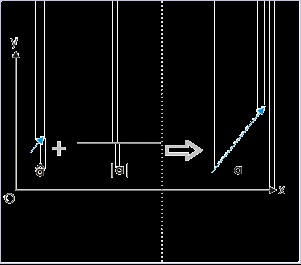
Unit vector has a magnitude of one and is directed in a particular direction. It does not have
dimension or unit like most other physical quantities. Thus, multiplying a scalar by unit vector
converts the scalar quantity into a vector without changing its magnitude, but assigning it a
direction ( Figure ).
Figure 1.32. Vector representation with unit vector
This is an important relation as it allows determination of unit vector in the direction of any
vector " a as :
Conventionally, unit vectors along the rectangular axes is represented with bold type face symbols
like : i , j and k , or with a cap heads like
. The unit vector along the axis denotes the
direction of individual axis.


Using the concept of unit vector, we can denote a vector by multiplying the magnitude of the
vector with unit vector in its direction.
Following this technique, we can represent a vector along any axis in terms of scalar magnitude
and axial unit vector like (for x-direction) :
a = a i
Other important vector terms
Null vector
Null vector is conceptualized for completing the development of vector algebra. We may
encounter situations in which two equal but opposite vectors are added. What would be the result?
Would it be a zero real number or a zero vector? It is expected that result of algebraic operation
should be compatible with the requirement of vector. In order to meet this requirement, we define
null vector, which has neither magnitude nor direction. In other words, we say that null vector is a
vector whose all components in rectangular coordinate system are zero.
Strictly, we should denote null vector like other vectors using a bold faced letter or a letter with an
overhead arrow. However, it may generally not be done. We take the exception to denote null
vector by number “0” as this representation does not contradicts the defining requirement of null
vector.
a + b = 0
Negative vector
Definition: Negative vector
A negative vector of a given vector is defined as the vector having same magnitude, but applied
in the opposite direction to that of the given vector.
It follows that if b is the negative of vector a , then
There is a subtle point to be made about negative scalar and vector quantities. A negative scalar
quantity, sometimes, conveys the meaning of lesser value. For example, the temperature -5 K is a
smaller temperature than any positive value. Also, a greater negative like – 100 K is less than the
smaller negative like -50 K. However, a scalar like charge conveys different meaning. A negative
charge of -10 μC is a bigger negative charge than – 5 μC. The interpretation of negative scalar is,
thus, situational.
On the other hand, negative vector always indicates the sense of opposite direction. Also like
charge, a greater negative vector is larger than smaller negative vector or a smaller positive
vector. The magnitude of force -10 i N, for example is greater than 5 i N, but directed in the
opposite direction to that of the unit vector i. In any case, negative vector does not convey the
meaning of lesser or greater magnitude like the meaning of a scalar quantity in some cases.
Co-planar vectors
A pair of vectors determines an unique plane. The pair of vectors defining the plane and other
vectors in that plane are called coplanar vectors.
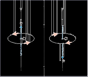
Axial vector
Motion has two basic types : translational and rotational motions. The vector and scalar quantities,
describing them are inherently different. Accordingly, there are two types of vectors to deal with
quantities having direction. The system of vectors that we have referred so far is suitable for