These are called cobalt γ rays, although they come from nickel—they are used for cancer therapy, for example. It is again constructive to verify the
conservation laws for gamma decay. Finally, since γ decay does not change the nuclide to another species, it is not prominently featured in charts of
decay series, such as that in Figure 31.16.
There are other types of nuclear decay, but they occur less commonly than α , β , and γ decay. Spontaneous fission is the most important of the
other forms of nuclear decay because of its applications in nuclear power and weapons. It is covered in the next chapter.
31.5 Half-Life and Activity
Unstable nuclei decay. However, some nuclides decay faster than others. For example, radium and polonium, discovered by the Curies, decay faster
than uranium. This means they have shorter lifetimes, producing a greater rate of decay. In this section we explore half-life and activity, the
quantitative terms for lifetime and rate of decay.
Half-Life
Why use a term like half-life rather than lifetime? The answer can be found by examining Figure 31.21, which shows how the number of radioactive
nuclei in a sample decreases with time. The time in which half of the original number of nuclei decay is defined as the half-life, t 1 / 2 . Half of the
remaining nuclei decay in the next half-life. Further, half of that amount decays in the following half-life. Therefore, the number of radioactive nuclei
decreases from N to N / 2 in one half-life, then to N / 4 in the next, and to N / 8 in the next, and so on. If N is a large number, then many half-lives (not just two) pass before all of the nuclei decay. Nuclear decay is an example of a purely statistical process. A more precise definition of half-life
is that each nucleus has a 50% chance of living for a time equal to one half-life t1 / 2 . Thus, if N is reasonably large, half of the original nuclei decay
in a time of one half-life. If an individual nucleus makes it through that time, it still has a 50% chance of surviving through another half-life. Even if it
happens to make it through hundreds of half-lives, it still has a 50% chance of surviving through one more. The probability of decay is the same no
matter when you start counting. This is like random coin flipping. The chance of heads is 50%, no matter what has happened before.
Figure 31.21 Radioactive decay reduces the number of radioactive nuclei over time. In one half-life t 1 / 2 , the number decreases to half of its original value. Half of what remains decay in the next half-life, and half of those in the next, and so on. This is an exponential decay, as seen in the graph of the number of nuclei present as a function of
time.
There is a tremendous range in the half-lives of various nuclides, from as short as 10−23 s for the most unstable, to more than 1016 y for the least
unstable, or about 46 orders of magnitude. Nuclides with the shortest half-lives are those for which the nuclear forces are least attractive, an
1128 CHAPTER 31 | RADIOACTIVITY AND NUCLEAR PHYSICS
indication of the extent to which the nuclear force can depend on the particular combination of neutrons and protons. The concept of half-life is
applicable to other subatomic particles, as will be discussed in Particle Physics. It is also applicable to the decay of excited states in atoms and nuclei. The following equation gives the quantitative relationship between the original number of nuclei present at time zero ( N 0 ) and the number (
N ) at a later time t :
(31.36)
N = N 0 e− λt,
where e = 2.71828... is the base of the natural logarithm, and λ is the decay constant for the nuclide. The shorter the half-life, the larger is the
value of λ , and the faster the exponential e− λt decreases with time. The relationship between the decay constant λ and the half-life t 1 / 2 is (31.37)
λ = ln(2)
t
≈ 0.693.
1/2
t 1/2
To see how the number of nuclei declines to half its original value in one half-life, let t = t 1 / 2 in the exponential in the equation N = N 0 e− λt . This gives N = N 0 e− λt = N 0 e−0.693 = 0.500 N 0 . For integral numbers of half-lives, you can just divide the original number by 2 over and over again, rather than using the exponential relationship. For example, if ten half-lives have passed, we divide N by 2 ten times. This reduces it to N / 1024 .
For an arbitrary time, not just a multiple of the half-life, the exponential relationship must be used.
Radioactive dating is a clever use of naturally occurring radioactivity. Its most famous application is carbon-14 dating. Carbon-14 has a half-life of
5730 years and is produced in a nuclear reaction induced when solar neutrinos strike 14 N in the atmosphere. Radioactive carbon has the same
chemistry as stable carbon, and so it mixes into the ecosphere, where it is consumed and becomes part of every living organism. Carbon-14 has an
abundance of 1.3 parts per trillion of normal carbon. Thus, if you know the number of carbon nuclei in an object (perhaps determined by mass and
Avogadro’s number), you multiply that number by 1.3 × 10⁻¹² to find the number of 14 C nuclei in the object. When an organism dies, carbon
exchange with the environment ceases, and 14 C is not replenished as it decays. By comparing the abundance of 14 C in an artifact, such as
mummy wrappings, with the normal abundance in living tissue, it is possible to determine the artifact’s age (or time since death). Carbon-14 dating
can be used for biological tissues as old as 50 or 60 thousand years, but is most accurate for younger samples, since the abundance of 14 C nuclei
in them is greater. Very old biological materials contain no 14 C at all. There are instances in which the date of an artifact can be determined by
other means, such as historical knowledge or tree-ring counting. These cross-references have confirmed the validity of carbon-14 dating and
permitted us to calibrate the technique as well. Carbon-14 dating revolutionized parts of archaeology and is of such importance that it earned the
1960 Nobel Prize in chemistry for its developer, the American chemist Willard Libby (1908–1980).
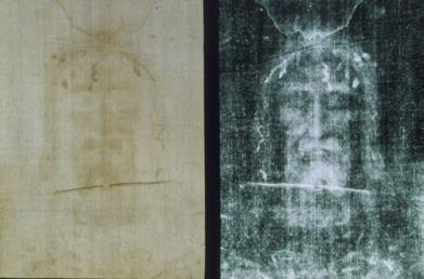
One of the most famous cases of carbon-14 dating involves the Shroud of Turin, a long piece of fabric purported to be the burial shroud of Jesus (see
Figure 31.22). This relic was first displayed in Turin in 1354 and was denounced as a fraud at that time by a French bishop. Its remarkable negative imprint of an apparently crucified body resembles the then-accepted image of Jesus, and so the shroud was never disregarded completely and
remained controversial over the centuries. Carbon-14 dating was not performed on the shroud until 1988, when the process had been refined to the
point where only a small amount of material needed to be destroyed. Samples were tested at three independent laboratories, each being given four
pieces of cloth, with only one unidentified piece from the shroud, to avoid prejudice. All three laboratories found samples of the shroud contain 92% of
the 14 C found in living tissues, allowing the shroud to be dated (see Example 31.4).
Figure 31.22 Part of the Shroud of Turin, which shows a remarkable negative imprint likeness of Jesus complete with evidence of crucifixion wounds. The shroud first surfaced
in the 14th century and was only recently carbon-14 dated. It has not been determined how the image was placed on the material. (credit: Butko, Wikimedia Commons)
Example 31.4 How Old Is the Shroud of Turin?
Calculate the age of the Shroud of Turin given that the amount of 14 C found in it is 92% of that in living tissue.
Strategy
CHAPTER 31 | RADIOACTIVITY AND NUCLEAR PHYSICS 1129
Knowing that 92% of the 14 C remains means that N / N 0 = 0.92 . Therefore, the equation N = N 0 e− λt can be used to find λt . We also know that the half-life of 14 C is 5730 y, and so once λt is known, we can use the equation λ = 0.693
t
to find λ and then find t as
1 / 2
requested. Here, we postulate that the decrease in 14 C is solely due to nuclear decay.
Solution
Solving the equation N = N 0 e− λt for N / N 0 gives
N
(31.38)
N = e− λt.
0
Thus,
(31.39)
0.92 = e− λt.
Taking the natural logarithm of both sides of the equation yields
(31.40)
ln 0.92 = –λt
so that
(31.41)
−0.0834 = − λt.
Rearranging to isolate t gives
(31.42)
t = 0.0834
λ .
Now, the equation λ = 0.693
t
can be used to find λ for 14 C . Solving for λ and substituting the known half-life gives
1 / 2
(31.43)
λ = 0.693
t
= 0.693
1 / 2
5730 y.
We enter this value into the previous equation to find t :
(31.44)
t = 0.0834
0.693 = 690 y.
5730 y
Discussion
This dates the material in the shroud to 1988–690 = a.d. 1300. Our calculation is only accurate to two digits, so that the year is rounded to 1300.
The values obtained at the three independent laboratories gave a weighted average date of a.d. 1320 ± 60 . The uncertainty is typical of
carbon-14 dating and is due to the small amount of 14 C in living tissues, the amount of material available, and experimental uncertainties
(reduced by having three independent measurements). It is meaningful that the date of the shroud is consistent with the first record of its
existence and inconsistent with the period in which Jesus lived.
There are other forms of radioactive dating. Rocks, for example, can sometimes be dated based on the decay of 238 U . The decay series for 238 U
ends with 206 Pb , so that the ratio of these nuclides in a rock is an indication of how long it has been since the rock solidified. The original
composition of the rock, such as the absence of lead, must be known with some confidence. However, as with carbon-14 dating, the technique can
be verified by a consistent body of knowledge. Since 238 U has a half-life of 4.5×10⁹ y, it is useful for dating only very old materials, showing, for
example, that the oldest rocks on Earth solidified about 3.5×10⁹ years ago.
Activity, the Rate of Decay
What do we mean when we say a source is highly radioactive? Generally, this means the number of decays per unit time is very high. We define
activity R to be the rate of decay expressed in decays per unit time. In equation form, this is
(31.45)
R = Δ N
Δ t
where Δ N is the number of decays that occur in time Δ t . The SI unit for activity is one decay per second and is given the name becquerel (Bq) in
honor of the discoverer of radioactivity. That is,
(31.46)
1 Bq = 1 decay/s.
Activity R is often expressed in other units, such as decays per minute or decays per year. One of the most common units for activity is the curie
(Ci), defined to be the activity of 1 g of 226 Ra , in honor of Marie Curie’s work with radium. The definition of curie is
1130 CHAPTER 31 | RADIOACTIVITY AND NUCLEAR PHYSICS
(31.47)
1 Ci = 3.70×10¹⁰ Bq,
or 3.70×10¹⁰ decays per second. A curie is a large unit of activity, while a becquerel is a relatively small unit. 1 MBq = 100 microcuries ( µ Ci) .
In countries like Australia and New Zealand that adhere more to SI units, most radioactive sources, such as those used in medical diagnostics or in
physics laboratories, are labeled in Bq or megabecquerel (MBq).
Intuitively, you would expect the activity of a source to depend on two things: the amount of the radioactive substance present, and its half-life. The
greater the number of radioactive nuclei present in the sample, the more will decay per unit of time. The shorter the half-life, the more decays per unit
time, for a given number of nuclei. So activity R should be proportional to the number of radioactive nuclei, N , and inversely proportional to their
half-life, t 1 / 2 . In fact, your intuition is correct. It can be shown that the activity of a source is
(31.48)
R = 0.693 N
t 1/2
where N is the number of radioactive nuclei present, having half-life t 1 / 2 . This relationship is useful in a variety of calculations, as the next two
examples illustrate.
Example 31.5 How Great Is the 14 C Activity in Living Tissue?
Calculate the activity due to 14 C in 1.00 kg of carbon found in a living organism. Express the activity in units of Bq and Ci.
Strategy
To find the activity R using the equation R = 0.693 N
t
, we must know N and t
1 / 2
1 / 2 . The half-life of 14 C can be found in Appendix B, and
was stated above as 5730 y. To find N , we first find the number of 12 C nuclei in 1.00 kg of carbon using the concept of a mole. As indicated,
we then multiply by 1.3 × 10⁻¹² (the abundance of 14 C in a carbon sample from a living organism) to get the number of 14 C nuclei in a
living organism.
Solution
One mole of carbon has a mass of 12.0 g, since it is nearly pure 12 C . (A mole has a mass in grams equal in magnitude to A found in the
periodic table.) Thus the number of carbon nuclei in a kilogram is
(31.49)
N(12 C) = 6.02×10²³ mol–1
12.0 g/mol
×(1000 g) = 5.02×1025 .
So the number of 14 C nuclei in 1 kg of carbon is
(31.50)
N(14 C) = (5.02×1025)(1.3×10⁻¹²) = 6.52×10¹³.
Now the activity R is found using the equation R = 0.693 N
t
.
1 / 2
Entering known values gives
(31.51)
R = 0.693(6.52 × 10¹³)
5730 y
= 7.89 × 10⁹ y–1,
or 7.89×10⁹ decays per year. To convert this to the unit Bq, we simply convert years to seconds. Thus,
(31.52)
R = (7.89 × 10⁹ y–1) 1.00 y
= 250 Bq,
3.16 × 10⁷ s
or 250 decays per second. To express R in curies, we use the definition of a curie,
(31.53)
R =
250 Bq
= 6.76 × 10⁻⁹ Ci.
3.7 × 10¹⁰ Bq/Ci
Thus,
R
(31.54)
= 6.76 nCi.
Discussion
Our own bodies contain kilograms of carbon, and it is intriguing to think there are hundreds of 14 C decays per second taking place in us.
Carbon-14 and other naturally occurring radioactive substances in our bodies contribute to the background radiation we receive. The small
number of decays per second found for a kilogram of carbon in this example gives you some idea of how difficult it is to detect 14 C in a small
sample of material. If there are 250 decays per second in a kilogram, then there are 0.25 decays per second in a gram of carbon in living tissue.

CHAPTER 31 | RADIOACTIVITY AND NUCLEAR PHYSICS 1131
To observe this, you must be able to distinguish decays from other forms of radiation, in order to reduce background noise. This becomes more
difficult with an old tissue sample, since it contains less 14 C , and for samples more than 50 thousand years old, it is impossible.
Human-made (or artificial) radioactivity has been produced for decades and has many uses. Some of these include medical therapy for cancer,
medical imaging and diagnostics, and food preservation by irradiation. Many applications as well as the biological effects of radiation are explored in
Medical Applications of Nuclear Physics, but it is clear that radiation is hazardous. A number of tragic examples of this exist, one of the most
disastrous being the meltdown and fire at the Chernobyl reactor complex in the Ukraine (see Figure 31.23). Several radioactive isotopes were
released in huge quantities, contaminating many thousands of square kilometers and directly affecting hundreds of thousands of people. The most
significant releases were of 131 I , 90 Sr , 137 Cs , 239 Pu , 238 U , and 235 U . Estimates are that the total amount of radiation released was about
100 million curies.
Human and Medical Applications
Figure 31.23 The Chernobyl reactor. More than 100 people died soon after its meltdown, and there will be thousands of deaths from radiation-induced cancer in the future.
While the accident was due to a series of human errors, the cleanup efforts were heroic. Most of the immediate fatalities were firefighters and reactor personnel. (credit: Elena
Filatova)
Example 31.6 What Mass of 137 Cs Escaped Chernobyl?
It is estimated that the Chernobyl disaster released 6.0 MCi of 137 Cs into the environment. Calculate the mass of 137 Cs released.
Strategy
We can calculate the mass released using Avogadro’s number and the concept of a mole if we can first find the number of nuclei N released.
Since the activity R is given, and the half-life of 137 Cs is found in Appendix B to be 30.2 y, we can use the equation R = 0.693 N
t
to find N
1 / 2
.
Solution
Solving the equation R = 0.693 N
t
for N gives
1 / 2
(31.55)
N = Rt 1/2
0.693.
Entering the given values yields
(31.56)
N = (6.0 MCi)(30.2 y)
0.693
.
Converting curies to becquerels and years to seconds, we get
(31.57)
N = (6.0 × 10⁶ Ci)(3.7 × 10¹⁰ Bq/Ci)(30.2 y)(3.16 × 10⁷ s/y)
0.693
= 3.1×1026 .
One mole of a nuclide A X has a mass of A grams, so that one mole of 137 Cs has a mass of 137 g. A mole has 6.02×10²³ nuclei. Thus
the mass of 137 Cs released was
(31.58)
m = ⎛ 137 g ⎞
⎝6.02×10²³⎠(3.1×1026) = 70×103 g
= 70 kg.

1132 CHAPTER 31 | RADIOACTIVITY AND NUCLEAR PHYSICS
Discussion
While 70 kg of material may not be a very large mass compared to the amount of fuel in a power plant, it is extremely radioactive, since it only
has a 30-year half-life. Six megacuries (6.0 MCi) is an extraordinary amount of activity but is only a fraction of what is produced in nuclear
reactors. Similar amounts of the other isotopes were also released at Chernobyl. Although the chances of such a disaster may have seemed
small, the consequences were extremely severe, requiring greater caution than was used. More will be said about safe reactor design in the next
chapter, but it should be noted that Western reactors have a fundamentally safer design.
Activity R decreases in time, going to half its original value in one half-life, then to one-fourth its original value in the next half-life, and so on. Since
R = 0.693 N
t
, the activity decreases as the number of radioactive nuclei decreases. The equation for R as a function of time is found by combining
1 / 2
the equations N = N 0 e− λt and R = 0.693 N
t
, yielding
1 / 2
(31.59)
R = R 0 e− λt,
where R 0 is the activity at t = 0 . This equation shows exponential decay of radioactive nuclei. For example, if a source originally has a 1.00-mCi
activity, it declines to 0.500 mCi in one half-life, to 0.250 mCi in two half-lives, to 0.125 mCi in three half-lives, and so on. For times other than whole
half-lives, the equation R = R 0 e− λt must be used to find R .
PhET Explorations: Alpha Decay
Watch alpha particles escape from a polonium nucleus, causing radioactive alpha decay. See how random decay times relate to the half life.
Figure 31.24 Alpha Decay (http://cnx.org/content/m42636/1.5/alpha-decay_en.jar)
31.6 Binding Energy
The more tightly bound a system is, the stronger the forces that hold it together and the greater the energy required to pull it apart. We can therefore
learn about nuclear forces by examining how tightly bound the nuclei are. We define the binding energy (BE) of a nucleus to be the energy required
to completely disassemble it into separate protons and neutrons. We can determine the BE of a nucleus from its rest mass. The two are connected
through Einstein’s famous relationship E = (Δ m) c 2 . A bound system has a smaller mass than its separate constituents; the more tightly the
nucleons are bound together, the smaller the mass of the nucleus.
Imagine pulling a nuclide apart as illustrated in Figure 31.25. Work done to overcome the nuclear forces holding the nucleus together puts energy
into the system. By definition, the energy input equals the binding energy BE. The pieces are at rest when separated, and so the energy put into them
increases their total rest mass compared with what it was when they were glued together as a nucleus. That mass increase is thus Δ m = BE / c 2 .
This difference in mass is known as mass defect. It implies that the mass of the nucleus is less than the sum of the masses of its constituent protons
and neutrons. A nuclide A X has Z protons and N neutrons, so that the difference in mass is
(31.60)
Δ m = ( Zmp + Nmn) − m tot.
Thus,
Describe what you're looking for in as much detail as you'd like.
Our AI reads your request and finds the best matching books for you.
Popular searches:
Join 2.9 million readers and get unlimited free ebooks