The hologram illustrated in Figure 30.45 is a transmission hologram. Holograms that are viewed with reflected light, such as the white light
holograms on credit cards, are reflection holograms and are more common. White light holograms often appear a little blurry with rainbow edges,
because the diffraction patterns of various colors of light are at slightly different locations due to their different wavelengths. Further uses of
holography include all types of 3-D information storage, such as of statues in museums and engineering studies of structures and 3-D images of
human organs. Invented in the late 1940s by Dennis Gabor (1900–1970), who won the 1971 Nobel Prize in Physics for his work, holography became
far more practical with the development of the laser. Since lasers produce coherent single-wavelength light, their interference patterns are more
pronounced. The precision is so great that it is even possible to record numerous holograms on a single piece of film by just changing the angle of
the film for each successive image. This is how the holograms that move as you walk by them are produced—a kind of lensless movie.
In a similar way, in the medical field, holograms have allowed complete 3-D holographic displays of objects from a stack of images. Storing these
images for future use is relatively easy. With the use of an endoscope, high-resolution 3-D holographic images of internal organs and tissues can be
made.
30.6 The Wave Nature of Matter Causes Quantization
After visiting some of the applications of different aspects of atomic physics, we now return to the basic theory that was built upon Bohr’s atom.
Einstein once said it was important to keep asking the questions we eventually teach children not to ask. Why is angular momentum quantized? You
already know the answer. Electrons have wave-like properties, as de Broglie later proposed. They can exist only where they interfere constructively,
and only certain orbits meet proper conditions, as we shall see in the next module.
Following Bohr’s initial work on the hydrogen atom, a decade was to pass before de Broglie proposed that matter has wave properties. The wave-like
properties of matter were subsequently confirmed by observations of electron interference when scattered from crystals. Electrons can exist only in
locations where they interfere constructively. How does this affect electrons in atomic orbits? When an electron is bound to an atom, its wavelength
must fit into a small space, something like a standing wave on a string. (See Figure 30.46.) Allowed orbits are those orbits in which an electron
constructively interferes with itself. Not all orbits produce constructive interference. Thus only certain orbits are allowed—the orbits are quantized.
Figure 30.46 (a) Waves on a string have a wavelength related to the length of the string, allowing them to interfere constructively. (b) If we imagine the string bent into a closed circle, we get a rough idea of how electrons in circular orbits can interfere constructively. (c) If the wavelength does not fit into the circumference, the electron interferes
destructively; it cannot exist in such an orbit.
For a circular orbit, constructive interference occurs when the electron’s wavelength fits neatly into the circumference, so that wave crests always
align with crests and wave troughs align with troughs, as shown in Figure 30.46 (b). More precisely, when an integral multiple of the electron’s
wavelength equals the circumference of the orbit, constructive interference is obtained. In equation form, the condition for constructive interference
and an allowed electron orbit is
nλ
(30.38)
n = 2 πrn( n = 1, 2, 3 ...),
where λn is the electron’s wavelength and rn is the radius of that circular orbit. The de Broglie wavelength is λ = h / p = h / mv , and so here λ = h / mev . Substituting this into the previous condition for constructive interference produces an interesting result:
CHAPTER 30 | ATOMIC PHYSICS 1089
nh
(30.39)
me v = 2π rn .
Rearranging terms, and noting that L = mvr for a circular orbit, we obtain the quantization of angular momentum as the condition for allowed orbits:
(30.40)
L = mevrn = n h
2π( n = 1, 2, 3 ...).
This is what Bohr was forced to hypothesize as the rule for allowed orbits, as stated earlier. We now realize that it is the condition for constructive
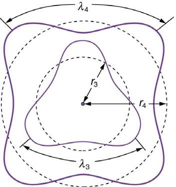
interference of an electron in a circular orbit. Figure 30.47 illustrates this for n = 3 and n = 4.
Waves and Quantization
The wave nature of matter is responsible for the quantization of energy levels in bound systems. Only those states where matter interferes
constructively exist, or are “allowed.” Since there is a lowest orbit where this is possible in an atom, the electron cannot spiral into the nucleus. It
cannot exist closer to or inside the nucleus. The wave nature of matter is what prevents matter from collapsing and gives atoms their sizes.
Figure 30.47 The third and fourth allowed circular orbits have three and four wavelengths, respectively, in their circumferences.
Because of the wave character of matter, the idea of well-defined orbits gives way to a model in which there is a cloud of probability, consistent with
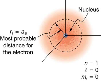
Heisenberg’s uncertainty principle. Figure 30.48 shows how this applies to the ground state of hydrogen. If you try to follow the electron in some well-defined orbit using a probe that has a small enough wavelength to get some details, you will instead knock the electron out of its orbit. Each
measurement of the electron’s position will find it to be in a definite location somewhere near the nucleus. Repeated measurements reveal a cloud of
probability like that in the figure, with each speck the location determined by a single measurement. There is not a well-defined, circular-orbit type of
distribution. Nature again proves to be different on a small scale than on a macroscopic scale.
Figure 30.48 The ground state of a hydrogen atom has a probability cloud describing the position of its electron. The probability of finding the electron is proportional to the darkness of the cloud. The electron can be closer or farther than the Bohr radius, but it is very unlikely to be a great distance from the nucleus.
There are many examples in which the wave nature of matter causes quantization in bound systems such as the atom. Whenever a particle is
confined or bound to a small space, its allowed wavelengths are those which fit into that space. For example, the particle in a box model describes a
particle free to move in a small space surrounded by impenetrable barriers. This is true in blackbody radiators (atoms and molecules) as well as in
atomic and molecular spectra. Various atoms and molecules will have different sets of electron orbits, depending on the size and complexity of the
system. When a system is large, such as a grain of sand, the tiny particle waves in it can fit in so many ways that it becomes impossible to see that
the allowed states are discrete. Thus the correspondence principle is satisfied. As systems become large, they gradually look less grainy, and
quantization becomes less evident. Unbound systems (small or not), such as an electron freed from an atom, do not have quantized energies, since
their wavelengths are not constrained to fit in a certain volume.

1090 CHAPTER 30 | ATOMIC PHYSICS
PhET Explorations: Quantum Wave Interference
When do photons, electrons, and atoms behave like particles and when do they behave like waves? Watch waves spread out and interfere as
they pass through a double slit, then get detected on a screen as tiny dots. Use quantum detectors to explore how measurements change the
waves and the patterns they produce on the screen.
Figure 30.49 Quantum Wave Interference (http://cnx.org/content/m42606/1.3/quantum-wave-interference_en.jar)
30.7 Patterns in Spectra Reveal More Quantization
High-resolution measurements of atomic and molecular spectra show that the spectral lines are even more complex than they first appear. In this
section, we will see that this complexity has yielded important new information about electrons and their orbits in atoms.
In order to explore the substructure of atoms (and knowing that magnetic fields affect moving charges), the Dutch physicist Hendrik Lorentz
(1853–1930) suggested that his student Pieter Zeeman (1865–1943) study how spectra might be affected by magnetic fields. What they found
became known as the Zeeman effect, which involved spectral lines being split into two or more separate emission lines by an external magnetic
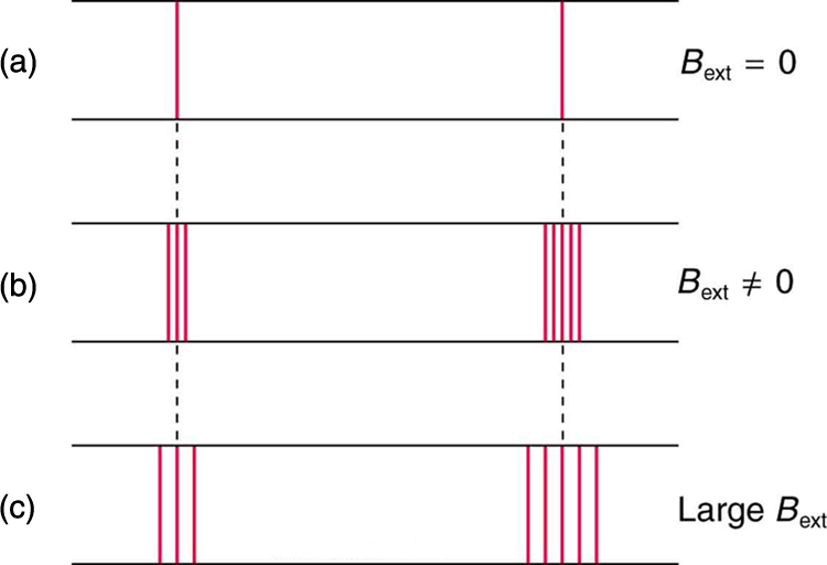
field, as shown in Figure 30.50. For their discoveries, Zeeman and Lorentz shared the 1902 Nobel Prize in Physics.
Zeeman splitting is complex. Some lines split into three lines, some into five, and so on. But one general feature is that the amount the split lines are
separated is proportional to the applied field strength, indicating an interaction with a moving charge. The splitting means that the quantized energy of
an orbit is affected by an external magnetic field, causing the orbit to have several discrete energies instead of one. Even without an external
magnetic field, very precise measurements showed that spectral lines are doublets (split into two), apparently by magnetic fields within the atom
itself.
Figure 30.50 The Zeeman effect is the splitting of spectral lines when a magnetic field is applied. The number of lines formed varies, but the spread is proportional to the
strength of the applied field. (a) Two spectral lines with no external magnetic field. (b) The lines split when the field is applied. (c) The splitting is greater when a stronger field is applied.
Bohr’s theory of circular orbits is useful for visualizing how an electron’s orbit is affected by a magnetic field. The circular orbit forms a current loop,
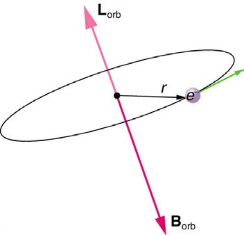
which creates a magnetic field of its own, Borb as seen in Figure 30.51. Note that the orbital magnetic field Borb and the orbital angular momentum Lorb are along the same line. The external magnetic field and the orbital magnetic field interact; a torque is exerted to align them. A
torque rotating a system through some angle does work so that there is energy associated with this interaction. Thus, orbits at different angles to the
external magnetic field have different energies. What is remarkable is that the energies are quantized—the magnetic field splits the spectral lines into
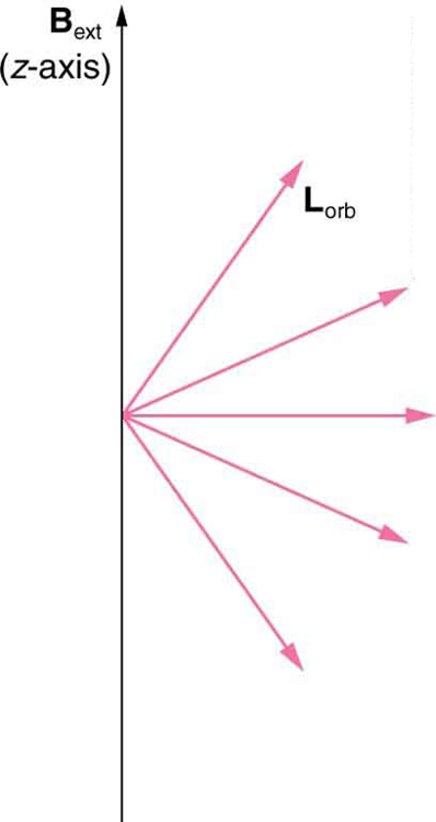
several discrete lines that have different energies. This means that only certain angles are allowed between the orbital angular momentum and the
external field, as seen in Figure 30.52.
CHAPTER 30 | ATOMIC PHYSICS 1091
Figure 30.51 The approximate picture of an electron in a circular orbit illustrates how the current loop produces its own magnetic field, called Borb . It also shows how Borb is along the same line as the orbital angular momentum Lorb .
Figure 30.52 Only certain angles are allowed between the orbital angular momentum and an external magnetic field. This is implied by the fact that the Zeeman effect splits
spectral lines into several discrete lines. Each line is associated with an angle between the external magnetic field and magnetic fields due to electrons and their orbits.
We already know that the magnitude of angular momentum is quantized for electron orbits in atoms. The new insight is that the direction of the orbital
angular momentum is also quantized. The fact that the orbital angular momentum can have only certain directions is called space quantization. Like
many aspects of quantum mechanics, this quantization of direction is totally unexpected. On the macroscopic scale, orbital angular momentum, such
as that of the moon around the earth, can have any magnitude and be in any direction.
Detailed treatment of space quantization began to explain some complexities of atomic spectra, but certain patterns seemed to be caused by
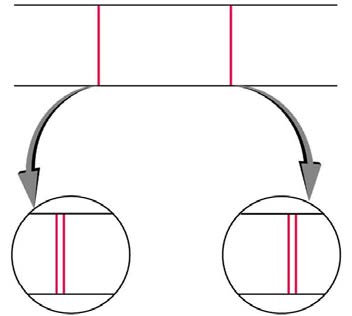
something else. As mentioned, spectral lines are actually closely spaced doublets, a characteristic called fine structure, as shown in Figure 30.53.
The doublet changes when a magnetic field is applied, implying that whatever causes the doublet interacts with a magnetic field. In 1925, Sem
Goudsmit and George Uhlenbeck, two Dutch physicists, successfully argued that electrons have properties analogous to a macroscopic charge
spinning on its axis. Electrons, in fact, have an internal or intrinsic angular momentum called intrinsic spin S . Since electrons are charged, their
intrinsic spin creates an intrinsic magnetic field Bint , which interacts with their orbital magnetic field Borb . Furthermore, electron intrinsic spin is
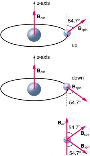
quantized in magnitude and direction, analogous to the situation for orbital angular momentum. The spin of the electron can have only one
magnitude, and its direction can be at only one of two angles relative to a magnetic field, as seen in Figure 30.54. We refer to this as spin up or spin down for the electron. Each spin direction has a different energy; hence, spectroscopic lines are split into two. Spectral doublets are now understood
as being due to electron spin.
1092 CHAPTER 30 | ATOMIC PHYSICS
Figure 30.53 Fine structure. Upon close examination, spectral lines are doublets, even in the absence of an external magnetic field. The electron has an intrinsic magnetic
field that interacts with its orbital magnetic field.
Figure 30.54 The intrinsic magnetic field Bint of an electron is attributed to its spin, S , roughly pictured to be due to its charge spinning on its axis. This is only a crude model, since electrons seem to have no size. The spin and intrinsic magnetic field of the electron can make only one of two angles with another magnetic field, such as that
created by the electron’s orbital motion. Space is quantized for spin as well as for orbital angular momentum.
These two new insights—that the direction of angular momentum, whether orbital or spin, is quantized, and that electrons have intrinsic spin—help to
explain many of the complexities of atomic and molecular spectra. In magnetic resonance imaging, it is the way that the intrinsic magnetic field of
hydrogen and biological atoms interact with an external field that underlies the diagnostic fundamentals.
30.8 Quantum Numbers and Rules
Physical characteristics that are quantized—such as energy, charge, and angular momentum—are of such importance that names and symbols are
given to them. The values of quantized entities are expressed in terms of quantum numbers, and the rules governing them are of the utmost
importance in determining what nature is and does. This section covers some of the more important quantum numbers and rules—all of which apply
in chemistry, material science, and far beyond the realm of atomic physics, where they were first discovered. Once again, we see how physics makes
discoveries which enable other fields to grow.
The energy states of bound systems are quantized, because the particle wavelength can fit into the bounds of the system in only certain ways. This
was elaborated for the hydrogen atom, for which the allowed energies are expressed as En ∝ 1/ n 2 , where n = 1, 2, 3, ... . We define n to be the
principal quantum number that labels the basic states of a system. The lowest-energy state has n = 1 , the first excited state has n = 2 , and so on.
Thus the allowed values for the principal quantum number are
n
(30.41)
= 1, 2, 3, ....
This is more than just a numbering scheme, since the energy of the system, such as the hydrogen atom, can be expressed as some function of n ,
as can other characteristics (such as the orbital radii of the hydrogen atom).
The fact that the magnitude of angular momentum is quantized was first recognized by Bohr in relation to the hydrogen atom; it is now known to be
true in general. With the development of quantum mechanics, it was found that the magnitude of angular momentum L can have only the values
CHAPTER 30 | ATOMIC PHYSICS 1093
(30.42)
L = l( l + 1) h
2π ( l = 0, 1, 2, ... , n − 1),
where l is defined to be the angular momentum quantum number. The rule for l in atoms is given in the parentheses. Given n , the value of l
can be any integer from zero up to n − 1 . For example, if n = 4 , then l can be 0, 1, 2, or 3.
Note that for n = 1 , l can only be zero. This means that the ground-state angular momentum for hydrogen is actually zero, not h / 2 π as Bohr
proposed. The picture of circular orbits is not valid, because there would be angular momentum for any circular orbit. A more valid picture is the cloud
of probability shown for the ground state of hydrogen in Figure 30.48. The electron actually spends time in and near the nucleus. The reason the
electron does not remain in the nucleus is related to Heisenberg’s uncertainty principle—the electron’s energy would have to be much too large to be
confined to the small space of the nucleus. Now the first excited state of hydrogen has n = 2 , so that l can be either 0 or 1, according to the rule in
L = l( l + 1) h
2π . Similarly, for n = 3 , l can be 0, 1, or 2. It is often most convenient to state the value of l , a simple integer, rather than
calculating the value of L from L = l( l + 1) h
2π . For example, for l = 2 , we see that
(30.43)
L = 2(2 + 1) h
2π = 6 h
2π = 0.390 h = 2.58×10⁻³⁴ J ⋅ s.
It is much simpler to state l = 2 .
As recognized in the Zeeman effect, the direction of angular momentum is quantized. We now know this is true in all circumstances. It is found that
the component of angular momentum along one direction in space, usually called the z -axis, can have only certain values of Lz . The direction in
space must be related to something physical, such as the direction of the magnetic field at that location. This is an aspect of relativity. Direction has
no meaning if there is nothing that varies with direction, as does magnetic force. The allowed values of Lz are
h ⎛
(30.44)
Lz = ml 2π ⎝ ml = − l, − l + 1, ... , − 1, 0, 1, ... l − 1, l⎞⎠,
where Lz is the z -component of the angular momentum and ml is the angular momentum projection quantum number. The rule in parentheses
for the values of ml is that it can range from − l to l in steps of one. For example, if l = 2 , then ml can have the five values –2, –1, 0, 1, and 2.
Each ml corresponds to a different energy in the presence of a magnetic field, so that they are related to the splitting of spectral lines into discrete
parts, as discussed in the preceding section. If the z -component of angular momentum can have only certain values, then the angular momentum
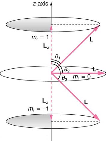
can have only certain directions, as illustrated in Figure 30.55.
Figure 30.55 The component of a given angular momentum along the z -axis (defined by the direction of a magnetic field) can have only certain values; these are shown here for l = 1 , for which ml = − 1, 0, and +1 . The direction of L is quantized in the sense that it can have only certain angles relative to the z -axis.
Example 30.3 What Are the Allowed Directions?
Calculate the angles that the angular momentum vector L can make with the z -axis for l = 1 , as illustrated in Figure 30.55.
Strategy
1094 CHAPTER 30 | ATOMIC PHYSICS
Figure 30.55 represents the vectors L and L z as usual, with arrows proportional to their magnitudes and pointing in the correct directions. L
and L z form a right triangle, with L being the hypotenuse and L z the adjacent side. This means that the ratio of L z to L is the cosine of the angle of interest. We can find L and L z using L = l( l + 1) h
2π and Lz = m h
2π .
Solution
We are given l = 1 , so that ml can be +1, 0, or −1. Thus L has the value given by L = l( l + 1) h
2π .
(30.45)
L = l( l + 1) h
2π
= 2 h
2π
L
h
z can have three values, given by Lz = ml 2π .
h
(30.46)
⎧⎪ 2π, ml = +1
L
h
z = ml 2π = ⎨ 0, m
⎪
l =
0
⎩− h
2π, ml = −1
As can be seen in Figure 30.55, cos θ = L z /L, and so for ml =+1 , we have
h
(30.47)
cos θ
2π
1 = LZ
L =
= 1 = 0.707.
2 h
2
2π
Thus,
(30.48)
θ 1 = cos−10.707 = 45.0º.
Similarly, for ml = 0 , we find cos θ 2 = 0 ; thus,
(30.49)
θ 2 = cos−10 = 90.0º.
And for ml = −1 ,
(30.50)
− h
cos θ
2π
3 = LZ
L =
= − 1 = −0.707,
Describe what you're looking for in as much detail as you'd like.
Our AI reads your request and finds the best matching books for you.
Popular searches:
Join 2.9 million readers and get unlimited free ebooks