College Physics (2012) by Manjula Sharma, Paul Peter Urone, et al - HTML preview
Download the book in PDF, ePub, Kindle for a complete version.
receives an opposite charge when charged by induction. Note also that no charge is removed from the charged rod, so that this process can be
repeated without depleting the supply of excess charge.
Another method of charging by induction is shown in Figure 18.14. The neutral metal sphere is polarized when a charged rod is brought near it. The
sphere is then grounded, meaning that a conducting wire is run from the sphere to the ground. Since the earth is large and most ground is a good
conductor, it can supply or accept excess charge easily. In this case, electrons are attracted to the sphere through a wire called the ground wire,
because it supplies a conducting path to the ground. The ground connection is broken before the charged rod is removed, leaving the sphere with an
excess charge opposite to that of the rod. Again, an opposite charge is achieved when charging by induction and the charged rod loses none of its
excess charge.
CHAPTER 18 | ELECTRIC CHARGE AND ELECTRIC FIELD 635
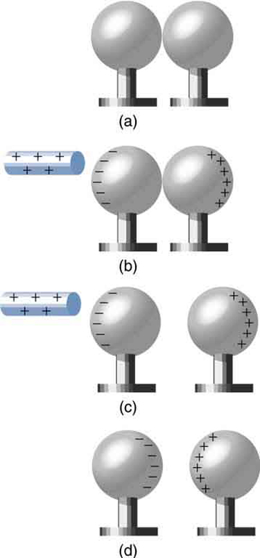
Figure 18.13 Charging by induction. (a) Two uncharged or neutral metal spheres are in contact with each other but insulated from the rest of the world. (b) A positively charged glass rod is brought near the sphere on the left, attracting negative charge and leaving the other sphere positively charged. (c) The spheres are separated before the rod is
removed, thus separating negative and positive charge. (d) The spheres retain net charges after the inducing rod is removed—without ever having been touched by a charged
object.
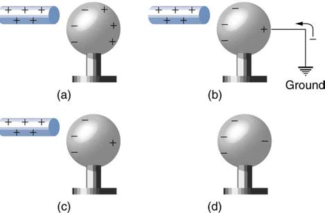
Figure 18.14 Charging by induction, using a ground connection. (a) A positively charged rod is brought near a neutral metal sphere, polarizing it. (b) The sphere is grounded,
allowing electrons to be attracted from the earth’s ample supply. (c) The ground connection is broken. (d) The positive rod is removed, leaving the sphere with an induced
negative charge.
636 CHAPTER 18 | ELECTRIC CHARGE AND ELECTRIC FIELD
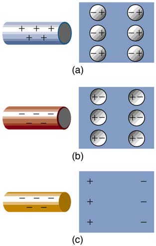
Figure 18.15 Both positive and negative objects attract a neutral object by polarizing its molecules. (a) A positive object brought near a neutral insulator polarizes its
molecules. There is a slight shift in the distribution of the electrons orbiting the molecule, with unlike charges being brought nearer and like charges moved away. Since the
electrostatic force decreases with distance, there is a net attraction. (b) A negative object produces the opposite polarization, but again attracts the neutral object. (c) The same
effect occurs for a conductor; since the unlike charges are closer, there is a net attraction.
Neutral objects can be attracted to any charged object. The pieces of straw attracted to polished amber are neutral, for example. If you run a plastic
comb through your hair, the charged comb can pick up neutral pieces of paper. Figure 18.15 shows how the polarization of atoms and molecules in
neutral objects results in their attraction to a charged object.
When a charged rod is brought near a neutral substance, an insulator in this case, the distribution of charge in atoms and molecules is shifted slightly.
Opposite charge is attracted nearer the external charged rod, while like charge is repelled. Since the electrostatic force decreases with distance, the
repulsion of like charges is weaker than the attraction of unlike charges, and so there is a net attraction. Thus a positively charged glass rod attracts
neutral pieces of paper, as will a negatively charged rubber rod. Some molecules, like water, are polar molecules. Polar molecules have a natural or
inherent separation of charge, although they are neutral overall. Polar molecules are particularly affected by other charged objects and show greater
polarization effects than molecules with naturally uniform charge distributions.
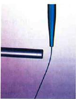
Can you explain the attraction of water to the charged rod in the figure below?
Figure 18.16
Solution
Water molecules are polarized, giving them slightly positive and slightly negative sides. This makes water even more susceptible to a charged
rod’s attraction. As the water flows downward, due to the force of gravity, the charged conductor exerts a net attraction to the opposite charges in
the stream of water, pulling it closer.

CHAPTER 18 | ELECTRIC CHARGE AND ELECTRIC FIELD 637
PhET Explorations: John Travoltage
Make sparks fly with John Travoltage. Wiggle Johnnie's foot and he picks up charges from the carpet. Bring his hand close to the door knob and
get rid of the excess charge.
Figure 18.17 John Travoltage (http://cnx.org/content/m42306/1.4/travoltage_en.jar)
18.3 Coulomb’s Law
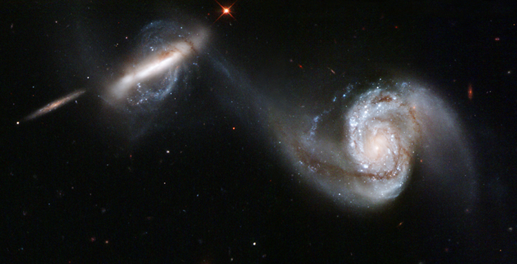
Figure 18.18 This NASA image of Arp 87 shows the result of a strong gravitational attraction between two galaxies. In contrast, at the subatomic level, the electrostatic
attraction between two objects, such as an electron and a proton, is far greater than their mutual attraction due to gravity. (credit: NASA/HST)
Through the work of scientists in the late 18th century, the main features of the electrostatic force—the existence of two types of charge, the
observation that like charges repel, unlike charges attract, and the decrease of force with distance—were eventually refined, and expressed as a
mathematical formula. The mathematical formula for the electrostatic force is called Coulomb’s law after the French physicist Charles Coulomb
(1736–1806), who performed experiments and first proposed a formula to calculate it.
Coulomb’s Law
(18.3)
F = k| q 1 q 2|
r 2 .
Coulomb’s law calculates the magnitude of the force F between two point charges, q 1 and q 2 , separated by a distance r . In SI units, the
constant k is equal to
(18.4)
k = 8.988×10⁹N ⋅ m2
C2 ≈ 9.00×10⁹N ⋅ m2
C2 .
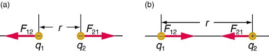
The electrostatic force is a vector quantity and is expressed in units of newtons. The force is understood to be along the line joining the two
charges. (See Figure 18.19.)
Although the formula for Coulomb’s law is simple, it was no mean task to prove it. The experiments Coulomb did, with the primitive equipment then
available, were difficult. Modern experiments have verified Coulomb’s law to great precision. For example, it has been shown that the force is
inversely proportional to distance between two objects squared ⎛⎝ F ∝ 1 / r 2⎞⎠ to an accuracy of 1 part in 1016 . No exceptions have ever been found,
even at the small distances within the atom.
Figure 18.19 The magnitude of the electrostatic force F between point charges q 1 and q 2 separated by a distance r is given by Coulomb’s law. Note that Newton’s third law (every force exerted creates an equal and opposite force) applies as usual—the force on q 1 is equal in magnitude and opposite in direction to the force it exerts on q 2 . (a) Like charges. (b) Unlike charges.
638 CHAPTER 18 | ELECTRIC CHARGE AND ELECTRIC FIELD
Example 18.1 How Strong is the Coulomb Force Relative to the Gravitational Force?
Compare the electrostatic force between an electron and proton separated by 0.530×10⁻¹⁰ m with the gravitational force between them. This
distance is their average separation in a hydrogen atom.
Strategy
To compare the two forces, we first compute the electrostatic force using Coulomb’s law, F = k| q 1 q 2|
r 2 . We then calculate the gravitational
force using Newton’s universal law of gravitation. Finally, we take a ratio to see how the forces compare in magnitude.
Solution
Entering the given and known information about the charges and separation of the electron and proton into the expression of Coulomb’s law
yields
(18.5)
F = k| q 1 q 2|
r 2
(18.6)
= ⎛⎝9.00×10⁹ N ⋅ m2 / C2⎞⎠×(1.60×10⁻¹⁹ C)(1.60×10⁻¹⁹ C)
(0.530×10⁻¹⁰ m)2
Thus the Coulomb force is
(18.7)
F = 8.20×10⁻⁸ N.
The charges are opposite in sign, so this is an attractive force. This is a very large force for an electron—it would cause an acceleration of
9.00×10²² m / s2 (verification is left as an end-of-section problem).The gravitational force is given by Newton’s law of gravitation as:
(18.8)
FG = GmM
r 2 ,
where G = 6.67×10⁻¹¹ N ⋅ m2 / kg2 . Here m and M represent the electron and proton masses, which can be found in the appendices.
Entering values for the knowns yields
(18.9)
FG = (6.67×10 – 11 N ⋅ m2 / kg2)×(9.11×10–31 kg)(1.67×10⁻²⁷ kg)
(0.530×10⁻¹⁰ m)2
= 3.61×10–47 N
This is also an attractive force, although it is traditionally shown as positive since gravitational force is always attractive. The ratio of the
magnitude of the electrostatic force to gravitational force in this case is, thus,
F
(18.10)
F = 2.27×1039.
G
Discussion
This is a remarkably large ratio! Note that this will be the ratio of electrostatic force to gravitational force for an electron and a proton at any
distance (taking the ratio before entering numerical values shows that the distance cancels). This ratio gives some indication of just how much
larger the Coulomb force is than the gravitational force between two of the most common particles in nature.
As the example implies, gravitational force is completely negligible on a small scale, where the interactions of individual charged particles are
important. On a large scale, such as between the Earth and a person, the reverse is true. Most objects are nearly electrically neutral, and so
attractive and repulsive Coulomb forces nearly cancel. Gravitational force on a large scale dominates interactions between large objects because it
is always attractive, while Coulomb forces tend to cancel.
18.4 Electric Field: Concept of a Field Revisited
Contact forces, such as between a baseball and a bat, are explained on the small scale by the interaction of the charges in atoms and molecules in
close proximity. They interact through forces that include the Coulomb force. Action at a distance is a force between objects that are not close
enough for their atoms to “touch.” That is, they are separated by more than a few atomic diameters.
For example, a charged rubber comb attracts neutral bits of paper from a distance via the Coulomb force. It is very useful to think of an object being
surrounded in space by a force field. The force field carries the force to another object (called a test object) some distance away.
Concept of a Field
A field is a way of conceptualizing and mapping the force that surrounds any object and acts on another object at a distance without apparent
physical connection. For example, the gravitational field surrounding the earth (and all other masses) represents the gravitational force that would be
experienced if another mass were placed at a given point within the field.
CHAPTER 18 | ELECTRIC CHARGE AND ELECTRIC FIELD 639
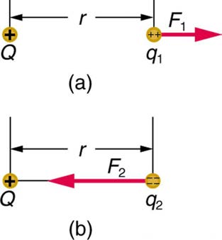
In the same way, the Coulomb force field surrounding any charge extends throughout space. Using Coulomb’s law, F = k| q 1 q 2| / r 2 , its magnitude is given by the equation F = k| qQ| / r 2 , for a point charge (a particle having a charge Q ) acting on a test charge q at a distance r (see Figure
18.20). Both the magnitude and direction of the Coulomb force field depend on Q and the test charge q .
Figure 18.20 The Coulomb force field due to a positive charge Q is shown acting on two different charges. Both charges are the same distance from Q . (a) Since q 1 is positive, the force F 1 acting on it is repulsive. (b) The charge q 2 is negative and greater in magnitude than q 1 , and so the force F 2 acting on it is attractive and stronger than F 1 . The Coulomb force field is thus not unique at any point in space, because it depends on the test charges q 1 and q 2 as well as the charge Q .
To simplify things, we would prefer to have a field that depends only on Q and not on the test charge q . The electric field is defined in such a
manner that it represents only the charge creating it and is unique at every point in space. Specifically, the electric field E is defined to be the ratio of
the Coulomb force to the test charge:
(18.11)
E = F q,
where F is the electrostatic force (or Coulomb force) exerted on a positive test charge q . It is understood that E is in the same direction as F . It
is also assumed that q is so small that it does not alter the charge distribution creating the electric field. The units of electric field are newtons per
coulomb (N/C). If the electric field is known, then the electrostatic force on any charge q is simply obtained by multiplying charge times electric field,
or F = qE . Consider the electric field due to a point charge Q . According to Coulomb’s law, the force it exerts on a test charge q is
F = k| qQ| / r 2 . Thus the magnitude of the electric field, E , for a point charge is
(18.12)
E = | Fq| = k| qQqr 2|= k| Q| r 2.
Since the test charge cancels, we see that
(18.13)
E = k| Q|
r 2 .
The electric field is thus seen to depend only on the charge Q and the distance r ; it is completely independent of the test charge q .
Example 18.2 Calculating the Electric Field of a Point Charge
Calculate the strength and direction of the electric field E due to a point charge of 2.00 nC (nano-Coulombs) at a distance of 5.00 mm from the
charge.
Strategy
We can find the electric field created by a point charge by using the equation E = kQ / r 2 .
Solution
Here Q = 2.00×10⁻⁹ C and r = 5.00×10⁻³ m. Entering those values into the above equation gives
(18.14)
E = k Q
r 2
= (9.00×10⁹ N ⋅ m2/C2 )× (2.00×10⁻⁹ C)
(5.00×10⁻³ m)2
= 7.20×10⁵ N/C.

640 CHAPTER 18 | ELECTRIC CHARGE AND ELECTRIC FIELD
Discussion
This electric field strength is the same at any point 5.00 mm away from the charge Q that creates the field. It is positive, meaning that it has a
direction pointing away from the charge Q .
Example 18.3 Calculating the Force Exerted on a Point Charge by an Electric Field
What force does the electric field found in the previous example exert on a point charge of –0.250 µ C ?
Strategy
Since we know the electric field strength and the charge in the field, the force on that charge can be calculated using the definition of electric field
E = F / q rearranged to F = qE .
Solution
The magnitude of the force on a charge q = −0.250 μC exerted by a field of strength E = 7.20×10⁵ N/C is thus,
F
(18.15)
= − qE
= (0.250×10⁻⁶ C)(7.20×10⁵ N/C)
= 0.180 N.
Because q is negative, the force is directed opposite to the direction of the field.
Discussion
The force is attractive, as expected for unlike charges. (The field was created by a positive charge and here acts on a negative charge.) The
charges in this example are typical of common static electricity, and the modest attractive force obtained is similar to forces experienced in static
cling and similar situations.
PhET Explorations: Electric Field of Dreams
Play ball! Add charges to the Field of Dreams and see how they react to the electric field. Turn on a background electric field and adjust the
direction and magnitude.
Figure 18.21 Electric Field of Dreams (http://cnx.org/content/m42310/1.5/efield_en.jar)
18.5 Electric Field Lines: Multiple Charges
Drawings using lines to represent electric fields around charged objects are very useful in visualizing field strength and direction. Since the electric
field has both magnitude and direction, it is a vector. Like all vectors, the electric field can be represented by an arrow that has length proportional to
its magnitude and that points in the correct direction. (We have used arrows extensively to represent force vectors, for example.)
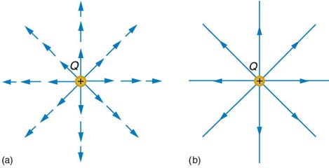
Figure 18.22 shows two pictorial representations of the same electric field created by a positive point charge Q . Figure 18.22 (b) shows the standard representation using continuous lines. Figure 18.22 (b) shows numerous individual arrows with each arrow representing the force on a test
charge q . Field lines are essentially a map of infinitesimal force vectors.
Figure 18.22 Two equivalent representations of the electric field due to a positive charge Q . (a) Arrows representing the electric field’s magnitude and direction. (b) In the standard representation, the arrows are replaced by continuous field lines having the same direction at any point as the electric field. The closeness of the lines is directly
related to the strength of the electric field. A test charge placed anywhere will feel a force in the direction of the field line; this force will have a strength proportional to the
density of the lines (being greater near the charge, for example).
CHAPTER 18 | ELECTRIC CHARGE AND ELECTRIC FIELD 641
Note that the electric field is defined for a positive test charge q , so that the field lines point away from a positive charge and toward a negative
charge. (See Figure 18.23.) The electric field strength is exactly proportional to the number of field lines per unit area, since the magnitude of the electric field for a point charge is E = k|Q| / r 2 and area is proportional to r 2 . This pictorial representation, in which field lines represent the direction and their closeness (that is, their areal density or the number of lines crossing a unit area) represents strength, is used for all fields:
electrostatic, gravitational, magnetic, and others.
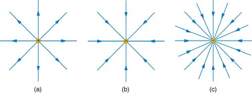
Figure 18.23 The electric field surrounding three different point charges. (a) A positive charge. (b) A negative charge of equal magnitude. (c) A larger negative charge.
In many situations, there are multiple charges. The total electric field created by multiple charges is the vector sum of the individual fields created by
each charge. The following example shows how to add electric field vectors.
Example 18.4 Adding Electric Fields
Find the magnitude and direction of the total electric field due to the two point charges, q 1 and q 2 , at the origin of the coordinate system as
shown in Figure 18.24.
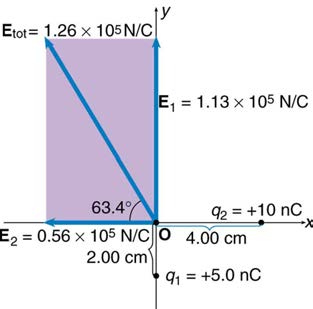
Figure 18.24 The electric fields E1 and E2 at the origin O add to Etot .
Strategy
Since the electric field is a vector (having magnitude and direction), we add electric fields with the same vector techniques used for other types of
vectors. We first must find the electric field due to each charge at the point of interest, which is the origin of the coordinate system (O) in this
instance. We pretend that there is a positive test charge, q , at point O, which allows us to determine the direction of the fields E1 and E2 .
Once those fields are found, the total field can be determined using vector addition.
Solution
The electric field strength at the origin due to q 1 is labeled E 1 and is calculated:
⎛
(18.16)
E
⎝5.00×10⁻⁹ C⎞⎠
1 = kq 1
r 2 = ⎛⎝9.00×10⁹ N ⋅ m2/C2⎞⎠
2
1
⎛⎝2.00×10⁻² m⎞⎠
E 1 = 1.125×10⁵ N/C.
Similarly, E 2 is
⎛
(18.17)
E
⎝10.0×10⁻⁹ C⎞⎠
2 = kq 2
r 2 = ⎛⎝9.00×10⁹ N ⋅ m2/C2⎞⎠
2
2
⎛⎝4.00×10⁻² m⎞⎠
E 2 = 0.5625×10⁵ N/C.
Four digits have been retained in this solution to illustrate that E 1 is exactly twice the magnitude of E 2 . Now arrows are drawn to represent the
magnitudes and directions of E1 and E2 . (See Figure 18.24.) The direction of the electric field is that of the force on a positive charge so both
642 CHAPTER 18 | ELECTRIC CHARGE AND ELECTRIC FIELD
arrows point directly away from the positive charges that create them. The arrow for E1 is exactly twice the length of that for E2 . The arrows
form a right triangle in this case and can be added using the Pythagorean theorem. The magnitude of the total field E tot is
2
2
(18.18)
E tot = ( E 1 + E 2 )1/2
= {(1.125×10⁵ N/C)2 + (0.5625×10⁵ N/C)2}1/2
= 1.26×10⁵ N/C.
The direction is
(18.19)
θ = tan−1⎛ E ⎞
<