

Classical Electrodynamics by Konstantin K. Likharev - HTML preview
Download the book in PDF, ePub, Kindle for a complete version.
where t is the 2D del operator acting in the transverse plane [ x, y] only, i.e. the usual , but with / z
= 0. The system (100) looks even bulkier than the original equations (2), but it is much simpler for analysis. Indeed, by eliminating the transverse components from these equations (or, even simpler, just by plugging Eq. (99) into Eqs. (3) and keeping only their z-components), we get a pair of self-consistent equations for the longitudinal components of the fields, 47
2D Helmholtz
equations for
2 2
k E
k
H
,
(7.101)
t
t
,
0
z
2 2
t
t
0
z
Ez and Hz
where k is still defined by Eq. (13), k ()1/2, while
Wave vector
component
2
2
2
2
2
k k k k
(7.102)
balance
t
z
z
After the distributions Ez( x,y) and Hz( x,y) have been found from these equations, they provide right-hand sides for the rather simple, closed system of equations (100) for the transverse components of field vectors. Moreover, as we will see below, each of the following three types of solutions: (i) with Ez = 0 and Hz = 0 (called the transverse electromagnetic, or TEM waves), (ii) with Ez = 0, but Hz 0 (called either the TE waves or, more frequently, H- modes), and (iii) with Ez 0, but Hz = 0 (the so-called TM waves or E- modes), has its own dispersion law and hence its own wave propagation velocity; as a result, these modes (i.e.
the field distribution patterns) may be considered separately.
In the balance of this section, we will focus on the simplest, TEM waves (i), with no longitudinal components of either field. For them, the top two equations of the system (100) immediately give Eqs.
(6) and (13), and kz = k. In plain English, this means that E = E t and H = H t are proportional to each other and are mutually perpendicular (just as in the plane wave) at each point of the cross-section and that the TEM wave’s impedance Z E/ H and dispersion law ( k), and hence the propagation speed, are the same as in a plane wave in the same material. In particular, if and are frequency-independent within a certain frequency range, the dispersion law within this range is linear, = k/()1/2, and the wave’s speed does not depend on its frequency. For practical applications to telecommunications, this is a very important advantage of the TEM waves over their TM and TE counterparts – to be discussed in the next sections.
Unfortunately for practice, such waves cannot propagate in every transmission line. To show this, let us have a look at the two last lines of Eqs. (100). For the TEM waves ( Ez = 0, Hz = 0, kz = k), they are reduced to merely
47 The wave equation represented in the form (101), even with the 3D Laplace operator, is called the Helmholtz equation, named after Hermann von Helmholtz (1821-1894) – the mentor of H. Hertz and M. Planck, among many others.
Chapter 7
Page 31 of 70


Essential Graduate Physics
EM: Classical Electrodynamics
E ,
0
H ,
0
t
t
t
t
(7.103)
E ,
0
H .
0
t
t
t
t
Within the coarse-grain description of the conducting walls of the line (i. e., neglecting not only the screening depth but also the skin depth in comparison with the cross-section dimensions), we have to require that inside them, E = H = 0. Close to a wall but outside it, the normal component En of the electric field may be different from zero, because surface charges may sustain its jump – see Sec. 2.1, in particular Eq. (2.3). Similarly, the tangential component H of the magnetic field may have a finite jump at the surface due to skin currents – see Sec. 6.3, in particular Eq. (6.38). However, the tangential component of the electric field and the normal component of the magnetic field cannot experience such jumps, and to have them equal to zero inside the walls they have to equal zero just outside the walls as well:
E ,
0
H 0
.
(7.104)
n
But the left columns of Eqs. (103)-(104) coincide with the formulation of the 2D boundary problem of electrostatics for the electric field induced by electric charges of the conducting walls, with the only difference that in our current case, the value of actually means (). Similarly, the right columns of those relations coincide with the formulation of the 2D boundary problem of magnetostatics for the magnetic field induced by currents in the walls, with (), with the only difference is that in our current coarse-grain approximation, the magnetic fields cannot penetrate into the conductors.
Now we immediately see that in waveguides with a singly-connected wall, for example, a hollow conducting tube (see, e.g., Fig. 16), the TEM waves are impossible, because there is no way to create a non-zero electrostatic field inside a conductor with such cross-section. However, such fields (and hence the TEM waves) are possible in structures with cross-sections consisting of two or more disconnected (galvanically-insulated) parts – see, e.g., Fig. 17.
H t
C
Fig. 7.17. An example of the cross-
section of a transmission line that may
support the TEM wave propagation.
E t
In order to derive “global” relations for such a transmission line, let us consider the contour C
drawn very close to the surface of one of its conductors – see, e.g., the red dashed line in Fig. 17. We can consider it, on one hand, as the cross-section of a cylindrically-shaped Gaussian volume of a certain elementary length dz << 2/ k. Using the generalized Gauss law (3.34), we get
E dr
,
(7.105)
t
n
C
where (not to be confused with the wavelength !) is the complex amplitude of the linear density of the electric charge of the conductor. On the other hand, the same contour C may be used in the generalized Ampère law (5.116) to write
Chapter 7
Page 32 of 70


Essential Graduate Physics
EM: Classical Electrodynamics
H
,
(7.106)
t dr
I
C
where I is the total current flowing along the conductor (or rather its complex amplitude). But, as was mentioned above, in the TEM wave the ratio Et/ Ht of the field components participating in these two integrals is constant and equal to Z = (/)1/2, so Eqs. (105)-(106) give the following simple relation between the “global” variables of the conductor:
/
I
.
(7.107)
Z
1/2
k
This important relation may be also obtained in a different way; let me describe it as well, because (as we will see below) it has an independent heuristic value. Let us consider a small segment dz
<< = 2/ k of the line’s conductor, and apply the electric charge conservation law (4.1) to the instant values of the linear charge density and current. The cancellation of dz in both parts yields
( z, t)
I
( z, t)
.
(7.108)
t
z
If we accept the sinusoidal waveform, exp{ i( kz – t)}, for both these variables, we immediately recover Eq. (107) for their complex amplitudes, showing that this relation expresses just the charge continuity law.
The global equation (108) may be made more specific in the case when the frequency dependence of and is negligible, and the transmission line consists of just two isolated conductors –
see, e.g., Fig. 17. In this case, to have the wave localized in the space near the two conductors, we need a sufficiently fast decrease of its electric field at large distances. For that, their linear charge densities for each value of z should be equal and opposite, and we can simply relate them to the potential difference V
between the conductors:
( z, t)
C ,
(7.109)
V ( z, t)
0
where C 0 is the mutual capacitance of the conductors (per unit length) – which was repeatedly discussed in Chapter 2. Then Eq. (108) takes the following form:
V
( z, t)
I
( z, t)
C
.
(7.110)
0
t
z
Next, let us consider the contour shown with the red dashed line in Fig. 18 (which shows a different cross-section of the transmission line – by a plane containing the wave propagation axis z), and apply to it the Faraday induction law (6.3).
I
I ( z, t)
I ( z, t)
dz
z
V
V ( z, t)
d L I ( z, t) dz
V ( z, t)
dz
0
z
Fig. 7.18. Electric current, magnetic flux, and
voltage in a two-conductor transmission line.
dz
Chapter 7
Page 33 of 70
EM: Classical Electrodynamics
Since, in the coarse-grain approximation, the electric field inside the conductors (in Fig. 18, on the horizontal segments of the contour) vanishes, the total e.m.f. equals the difference of the voltages V
at the ends of the segment dz, while the only sources of the magnetic flux through the area limited by the contour are the (equal and opposite) currents I in the conductors, we can use Eq. (5.70) to express the flux. As a result, by canceling dz in both parts of the equation, we get
I
( z, t)
V
( z, t)
L
,
(7.111)
0
t
z
where L 0 is the mutual inductance of the conductors per unit length. The only difference between this L 0
and the dc mutual inductances discussed in Chapter 5 is that at the high frequencies we are analyzing now, L 0 should be calculated neglecting the magnetic field penetration into the conductors. (In the dc case, we had the same situation for superconductor electrodes within their coarse-grain, ideal-diamagnet description.)
The system of Eqs. (110) and (111) is frequently called the telegrapher’s equations. Combined, they give for any “global” variable f (either V, or I, or ) the usual 1D wave equation, 2
2
f
f
L C
0 ,
(7.112)
2
0
0
2
z
t
which describes dispersion-free TEM wave’s propagation. Again, this equation is only valid within the frequency range where the frequency dependence of both and is negligible. If this is not so, the global approach may still be used for sinusoidal waves f = Re[ fexp{ i( kz – t)}]. Repeating the above arguments, instead of Eqs. (110)-(111) we get a more general system of two algebraic equations
C V kI ,
L I kV ,
(7.113)
0
0
in which L 0 and C 0 may now depend on frequency. These equations are consistent only if 2
k
1
L 0 C 0
L C
.
(7.114) product
0
0
2
2
v
invariance
Besides the fact we have already known (that the TEM wave’s speed is the same as that of the plane wave), Eq. (114) gives us the result that I confess was not emphasized enough in Chapter 5: the product L 0 C 0 does not depend on the shape or size of line’s cross-section, provided that the magnetic field’s penetration into the conductors is negligible). Hence, if we have calculated the mutual capacitance C 0 of a system of two cylindrical conductors, the result immediately gives us their mutual inductance: L 0 =
/ C 0. This relationship stems from the fact that both the electric and magnetic fields may be expressed via the solution of the same 2D Laplace equation for the system’s cross-section.
With Eq. (114) satisfied, any of Eqs. (113) gives the same result for the following ratio: 1/ 2
V
L
Transmission
0
Z
,
(7.115) line’s TEM
W
I
Impedance
C 0
which is called the transmission line’s impedance. This parameter has the same dimensionality (in SI units – ohms, denoted ) as the wave impedance (7),
Chapter 7
Page 34 of 70


Essential Graduate Physics
EM: Classical Electrodynamics
1/ 2
E
Z
,
(7.116)
H
but these parameters should not be confused, because ZW depends on the cross-section’s geometry, while Z does not. In particular, ZW is the only important parameter of a transmission line for its matching with a lumped load circuit (Fig. 19) in the important case when both the cable cross-section’s size and the load’s linear dimensions are much smaller than the wavelength.48
Z
I
W
Z ()
L
V
Fig. 7.19. Passive, lumped
termination of a TEM
transmission line.
z
z
0
Indeed, in this case, we may consider the load in the quasistatic limit and write
V ( z ) Z () I ( z )
,
(7.117)
0
L
0
where ZL() is the (generally complex) impedance of the load. Taking V( z,t) and I( z,t) in the form similar to Eqs. (61) and (62), and writing the two Kirchhoff’s circuit laws for the point z = z 0, we get for the reflection coefficient a result similar to Eq. (68):
Z () Z
L
W
R
.
(7.118)
Z () Z
L
W
This formula shows that for the perfect matching (i.e. the total wave absorption in the load), the load’s impedance ZL() should be real and equal to ZW – but not necessarily to Z.
As an example, let us consider one of the simplest (and most practically important) transmission lines: the coaxial cable (Fig. 20).49
, b a
0
a
Fig. 7. 20. The cross-section of a coaxial cable
with (possibly, dispersive) dielectric filling.
For this geometry, we already know the expressions for both C 0 and L 0,50 though they have to be modified for the account of arbitrary dielectric and magnetic constants, and the magnetic field’s non-penetration into the conductors. As a result of this (elementary) modification, we get the formulas, 48 The ability of TEM lines to have such a small cross-section is another important practical advantage.
49 It was invented by the same O. Heaviside in 1880.
50 See, respectively, Eqs. (2.49) and (5.79).
Chapter 7
Page 35 of 70
Essential Graduate Physics
EM: Classical Electrodynamics
2
Coaxial
C
,
L
ln( b / a) ,
(7.119) cable’s
0
ln( b / a)
0
2
C 0 and L 0
illustrating that the universal relationship (114) is indeed valid. For the cable’s impedance (115), Eqs.
(119) yield a geometry-dependent value
1/2
b
ln( / a)
b
ln( / a)
Z
Z
Z .
(7.120)
W
2
2
For the standard TV antenna cables (such as RG-6/U, with b/ a ~ 3, /0 2.2), ZW = 75 , while for most computer component connections, coaxial cables with ZW = 50 (such as RG-58/U) are prescribed by electronic engineering standards. Such cables are broadly used for the transmission of electromagnetic waves with frequencies up to 1 GHz over distances of a few km, and up to ~20 GHz on the tabletop scale (a few meters), limited by wave attenuation – see Sec. 9 below.
Moreover, the following two facts enable a wide application, in electrical engineering and physical experiment, of coaxial-cable- like systems. First, as Eq. (5.78) shows, in a cable with a << b, most energy of the wave is localized near the internal conductor. Second, the theory to be discussed in the next section shows that excitation of other ( H- and E-) waves in the cable is impossible until the wavelength becomes smaller than ~( a + b). As a result, the TEM mode propagation in a cable with a
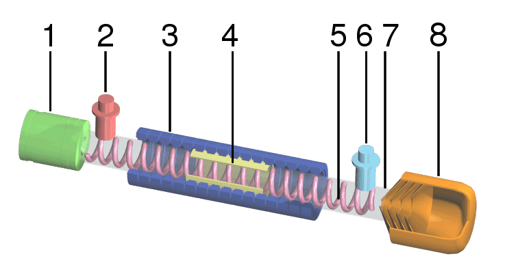
<< b < / is not much affected even if the internal conductor is not straight, but bent – for example, into a helix – see, e.g., Fig. 21.
Fig. 7.21. A typical traveling-wave tube:
(1) electron gun, (2) ac input, (3) beam-
focusing magnets, (4) wave attenuator,
(5) helix coil, (6) ac output, (7) vacuum
tube, (8) electron collector. Adapted from
https://en.wikipedia.org/wiki/Traveling-
wave_tube under the Creative Commons
BY-SA 3.0 license.
In such a system, called the traveling-wave tube (TWT), a quasi-TEM wave propagates with velocity v c along the helix’s length, so the velocity’s component along the cable’s axis may be made close to the velocity u << c of the electron beam moving ballistically along the tube’s axis, enabling their effective interaction, and as a result, a length-accumulating amplification of the wave.51
Another important example of a TEM transmission line is a set of two parallel wires. In the form of twisted pairs,52 they allow communications, in particular long-range telephone and DSL Internet 51 Despite the current prevalence of semiconductor devices in electronics, TWTs are still used in satellite TV and radio systems, because they may work at very high microwave power – e.g., up to 200W at 20
GHz and pulsed 50W at 200 GHz. Very unfortunately, in this course, I will not have time/space to discuss even the (rather elegant) basic theory of such devices. The reader interested in this field may be referred, for example, to the detailed monograph by J. Whitaker, Power Vacuum Tubes Handbook, 3rd ed., CRC Press, 2017.
52 Such twisting, around the line’s direction axis, reduces the crosstalk between adjacent lines, and the parasitic radiation at their bends.
Chapter 7
Page 36 of 70
EM: Classical Electrodynamics
connections, at frequencies up to a few hundred kHz, as well as relatively short, multi-line Ethernet and TV cables at frequencies up to ~ 1 GHz, limited mostly by the mutual interference (“crosstalk”) between the individual lines of the same cable, and the unintentional radiation of the wave into the environment.
7.6. Waveguides: H and E waves
Let us now return to Eqs. (100) and explore the H- and E-waves – with, respectively, either Hz or Ez different from zero. At the first sight, they may seem more complex. However, Eqs. (101), which determine the distribution of these longitudinal components over the cross-section, are just the 2D
Helmholtz equations for scalar functions. For simple cross-section geometries, they may be readily solved using the methods discussed for the Laplace equation in Chapter 2, in particular the variable separation. After the solution of such an equation has been found, the transverse components of the fields may be calculated by differentiation, using the simple formulas,
i
i
k
E
k E
kZ n
H
H
k H
n
E
(7.121)
t
(
)
z
t
z
z
t
z ,
(
) ,
2
t
2 z
t
z
z
t
z
k
k
Z
t
t
which follow from the first line of Eqs. (100).53
In comparison with the boundary problems of electro- and magnetostatics, the only conceptually new feature of Eqs. (101) is that they form the so-called eigenproblems, with typically many solutions ( eigenfunctions), each describing a specific wave mode, and corresponding to a specific eigenvalue of the parameter kt. The good news here is that these values of kt are determined by this 2D boundary problem and hence do not depend on kz. As a result, the dispersion law ( kz) of any mode, which follows from the last form of Eq. (102),
1/ 2
Universal
2
2
k k
dispersion
z
t
2 2
2
v k
,
(7.122)
z
c 1/ 2
relation
is functionally similar for all modes. It is also similar to that of plane waves in plasma (see Eq. (38), Fig.
6, and their discussion in Sec. 2), with the only difference that the speed in light c is generally replaced with v = 1/()1/2 – the speed of the plane or TEM waves in the medium filling the waveguide, and that
p is replaced with the so-called cutoff frequency
vk ,
(7.123)
c
t
specific for each mode. (As Eq. (101) implies, and as we will see from several examples below, kt has the order of 1/ a, where a is the characteristic dimension of the waveguide’s cross-section, so the critical value of the free-space wavelength 2 c/ is of the order of a.) Below the cutoff frequency of each particular mode, this wave cannot propagate in the waveguide.54 As a result, the modes with the lowest 53 For the derivation of Eqs. (121), one of these two linear equations should be first vector-multiplied by n z. Note also that this approach could not be used to analyze the TEM waves, because for them kt = 0, Ez = 0, Hz = 0, and Eqs. (121) yield uncertainty.
54 An interesting twist in the ideas of electromagnetic metamaterials (mentioned in Sec. 5 above) is the so-called
-near-zero materials, designed to have the effective product much lower than 00 within certain frequency ranges. Since at these frequencies, the speed v (4) becomes much lower than c, the cutoff frequency (123) Chapter 7
Page 37 of 70


Essential Graduate Physics
EM: Classical Electrodynamics
values of c present special practical interest, because the choice of the signal frequency between the two lowest values of the cutoff frequency (123) guarantees that the waves propagate in the form of only one mode, with the lowest kt. Such a choice enables engineers to simplify the excitation of the desired mode by wave generators and to avoid the unintentional transfer of electromagnetic wave energy to undesirable modes by (virtually unavoidable) small inhomogeneities of the system.
The boundary conditions for the Helmholtz equations (101) depend on the propagating wave type. For the E-modes, with Hz = 0 but Ez 0, the condition E = 0 immediately gives E
,
0
(7.124)
z C
where C is the inner contour limiting the conducting wall’s cross-section. For the H-modes, with Ez = 0
but Hz 0, the boundary condition is slightly less obvious and may be obtained using, for example, the second equation of the system (100), vector-multiplied by n z. Indeed, for the component normal to the conductor surface, the result of such multiplication is
k
H
ik (H ) i
n E
.
(7.125)
z
t n
z
t
z
Z
n
n
But the first term on the left-hand side of this relation must be zero on the wall surface, because of the second of Eqs. (104), while according to the first of Eqs. (104), the vector E t in the second term cannot have a component tangential to the wall. As a result, the vector product in that term cannot have a normal component, so the term should equal zero as well, and Eq. (125) is reduced to
H
z
0 .
(7.126)
C
n
Let us see how all this machinery works for a simple but practically important case of a metallic-wall waveguide with a rectangular cross-section – see Fig. 22
y
b
H t
Fig. 7.22. A rectangular waveguide, and the
E
transverse
field
distribution
in
its
0
a
fundamental mode H 10 (schematically).
x
In the natural Cartesian coordinates shown in this figure, both Eqs. (101) take the simple form
2
2
E , for E -
modes,
2
k
f ,
0
where f
z
(7.127)
2
2
t
x
y
H , for H - modes.
z
From Chapter 2, we know that the most effective way of solving such equations in a rectangular region is the variable separation, in which the general solution is represented as a sum of partial solutions of the type
virtually vanishes. As a result, the waves may “tunnel” through very narrow sections of metallic waveguides filled with such materials – see, e.g., M. Silveirinha and N. Engheta, Phys. Rev. Lett. 97, 157403 (2006).
Chapter 7
Page 38 of 70
EM: Classical Electrodynamics
f X ( x) Y ( y) .
(7.128)
Plugging this expression into Eq. (127), and dividing each term by XY, we get the equation, 1
2
d X
1 2
d Y
2
k 0,
(7.129)
2
2
t
X dx
Y dy
which should be satisfied for all values of x and y within the waveguide’s interior. This is only possible if each term of the sum equals a constant. Taking the X-term and Y-term constants in the form (– k 2
x ) and
(– k 2
y ), respectfully, and solving the corresponding ordinary differential equations,55 for the eigenfunction (128) we get
f c cos k x s sin k x c
k y s
k y
k k k ,
(7.130)
x
x
x
x
cos
sin
y
y
y
y
2
2
2
,
with x
y
t
where the constants c and s should be found from the boundary conditions. Here the difference between the H-modes and E-modes kicks in.
For the H-modes, Eq. (130) is valid for Hz, and we should use the boundary condition (126) on all metallic walls of the waveguide, i.e. at x = 0 and a; and y = 0 and b – see Fig. 22. As a result, we get very simple expressions for eigenfunctions and eigenvalues:
nx
my
H
cos
cos
,
(7.131)
z
H
nm
l
a
b
1/ 2
2
2
n
m
n
m
k
, k
,
(
that
so
k )
(7.132)
x
y
t nm
2 2
k k
x
y 1/ 2
,
a
b
a
b
where Hl is the longitudinal field’s amplitude, and n and m are two integer numbers – each of them arbitrary besides that they cannot be equal to zero simultaneously.56 Assuming, just for certainty, that a
b (as shown in Fig. 22), we see that the lowest eigenvalue of kt and hence the lowest cutoff frequency (123) are achieved for the so-called H 10 mode with n = 1 and m = 0, and hence with Fundamental
mode’s
( k )
,
(7.133)
t 10
cutoff
a
thus confirming our prior estimate of kt.
Depending on the a/ b ratio, the second-lowest kt (and hence c) belongs to either the H 11 mode with n = 1 and m = 1:
1/ 2
1/ 2
2
1
1
a
( k )
1
( k ) ,
(7.134)
t 11
2
2
t 10
a
b
b
or to the H 20 mode with n = 2 and m = 0:
55 Let me hope that the solution of equations of the type d 2 X/ dx 2 + k 2
x X = 0 does not present any problem for the
reader, at least due to their prior experience with problems such as standing waves on a guitar string, wavefunctions in a flat 1D quantum well, or (with the replacement x t) a classical harmonic oscillator.
56 Otherwise, the function Hz( x,y) would be constant, so, according to Eq. (121), the transverse components of the electric and magnetic field would equal zero. As a result, as the last two lines of Eqs. (100) show, the whole field would be zero for any kz 0.
Chapter 7
Page 39 of 70
EM: Classical Electrodynamics
2
( k )
(
2 k ) .
(7.135)
t 20
t 10
a
These values become equal at a/ b = 3 1.7; in practical waveguides, the a/ b ratio is not too far from this value. For example, in the standard X-band (~10-GHz) waveguide WR90, a 2.3 cm ( f c c/2
6.5 GHz), and b 1.0 cm.
Now let us have a look at the alternative E-modes. For them, we still should use the general solution (130) with f = Ez, but now with the boundary condition (124). This gives us the eigenfunctions
nx
my
E
sin
sin
,
(7.136)
z
E
nm
l
a
b
and the same eigenvalue spectrum (132) as for the H modes. However, now neither n nor m can be equal to zero; otherwise, Eq. (136) would give the trivial solution Ez( x,y) = 0. Hence the lowest cutoff frequency of TM waves is achieved at the so-called E 11 mode with n =1, m = 1, and with the eigenvalue given by Eq. (134), always higher than ( kt)10.
Thus the fundamental H 10 mode is certainly the most important wave in rectangular waveguides; let us have a better look at this field distribution. Plugging the corresponding solution (131) with n = 1
and m = 0 into the general relation (121), we easily get
k a
x
( H ) z
i
H sin
,
( H ) ,
0
(7.137)
x 10
l
y 10
a
ka
x
( E ) ,
0
( E ) i
ZH sin
.
(7.138)
x 10
y 10
l
a
This field distribution is (schematically) shown in Fig. 22. Neither of the fields depends on the coordinate y – the feature very convenient, in particular, for microwave experiments with small samples.
The electric field has only one (in Fig. 22, vertical) component that vanishes at the side walls and reaches its maximum at the waveguide’s center; its field lines are straight, starting and ending on wall surface charges (whose distribution propagates along the waveguide together with the wave). In contrast, the magnetic field has two non-zero components ( Hx and Hz), and its field lines are shaped as horizontal loops wrapped around the electric field maxima.
An important question is whether the H 10 wave may be usefully characterized by a unique impedance introduced similarly to ZW of the TEM modes – see Eq. (115). The answer is not, because the main value of ZW is a convenient description of the impedance matching of a transmission line with a lumped load – see Fig. 19 and Eq. (118). As was discussed above, such a simple description is possible (i.e., does not depend on the exact geometry of the connection) only if both dimensions of the line’s cross-section are much less than . But for the H 10 wave (and more generally, any non-TEM mode) this is impossible – see, e.g., Eq. (129): its lowest frequency corresponds to the TEM wavelength max =
2/( kt)min = 2/( kt)10 = 2 a. (The reader is challenged to find a simple interpretation of this equality.) Now let us consider metallic-wall waveguides with a round cross-section (Fig. 23a). In this single-connected geometry, the TEM waves are impossible again, while for the analysis of H-modes and E-modes, the polar coordinates {, } are most natural. In these coordinates, the 2D Helmholtz equation (101) takes the following form:
Chapter 7
Page 40 of 70


Essential Graduate Physics
EM: Classical Electrodynamics
1
1 2
E
E
2
, for - modes,
z
k
f
f
(7.139)
2
2
t
,
0
where
H , for H - modes.
z
Separating the variables as f = R() F(), we get
1 d dR
1
2
d
F
2
k 0
.
(7.140)
2
2
R d d
t
F d
But this is exactly the Eq. (2.127) that was studied in Sec. 2.7 in the context of electrostatics, just with a replacement of notation: kt. So we already know that to have 2-periodic functions F() and finite values R(0) (which are evidently necessary for our current case – see Fig. 23a), the general solution must have the form given by Eq. (2.136), i.e. the eigenfunctions are expressed via integer-order Bessel functions of the first kind:
f
J
,
(7.141)
nm
n k
nm
c cos
n s sin
n
n
n
const Jn k
nm
cos n 0
with the eigenvalues knm of the transverse wave number kt to be determined from appropriate boundary conditions, and an arbitrary constant 0.
(a)
(b)
,
R
,
R
0
0
Fig. 7.23. (a) Metallic and (b) dielectric
,
waveguides with circular cross-sections.
As for the rectangular waveguide, let us start with the H-modes ( f = Hz). Then the boundary condition on the wall surface ( = R) is given by Eq. (126), which, for the solution (141), takes the form d
J
( ) ,
0
where
kR .
(7.142)
d
n
This means that the eigenvalues of Eq. (139) are
'
k k
nm
,
(7.143)
t
nm
R
where ’nm is the m th zero of the function dJn()/ d. Approximate values of these zeros for several lowest n and m may be read out from Fig. 2.18; their more accurate values are given in Table 1 below.
Table 7.1. Zeros ’nm of the function dJn()/ d for a few lowest values of the Bessel function’s index n and the root’s number m.
m = 1
2
3
n = 0
3.83171
7.015587
10.1735
1
1.84118
5.33144
8.53632
2
3.05424
6.70613
9.96947
3
4.20119
8.01524
11.34592
Chapter 7
Page 41 of 70


Essential Graduate Physics
EM: Classical Electrodynamics
The table shows, in particular, that the lowest of the zeros is ’ 11 1.84.57 Thus, perhaps a bit counter-intuitively, the fundamental mode, providing the lowest cutoff frequency c = vknm, is H 11, corresponding to n = 1 rather than n = 0:
'
H H J
.
(7.144)
z
l
cos
1
11
0
R
It has the transverse wave number is kt = k 11 = ’ 11/ R 1.84/ R, and hence the cutoff frequency corresponding to the TEM wavelength max = 2/ k 11 3.41 R. Thus the ratio of max to the waveguide’s diameter 2 R is about 1.7, i.e. is close to the ratio max/ a = 2 for the rectangular waveguide. The origin of this proximity is clear from Fig. 24, which shows the transverse field distribution in the H 11 mode. (It may be readily calculated from Eqs. (121) with Ez = 0 and Hz given by Eq. (144).) E
H
Fig. 7.24. Transverse field components in the
fundamental H 11 mode of a metallic, circular
waveguide (schematically).
One can see that the field structure is actually very similar to that of the fundamental mode in the rectangular waveguide, shown in Fig. 22, despite the different nomenclature (which is due to the different coordinate system used for the solution). However, note the arbitrary constant angle 0, indicating that in circular waveguides, the transverse field’s polarization is arbitrary. For some practical applications, such degeneracy of these “quasi-linearly-polarized” waves creates problems; some of them may be avoided by using waves with circular polarization.
As Table 1 shows, the next lowest H-mode is H 21, for which kt = k 21 = ’ 21/ R 3.05/ R, almost twice larger than that of the fundamental mode, and only then comes the first mode with no angular dependence of any field, H 01, with kt = k 01 = ’ 01/ R 3.83/ R,58 followed by several angle-dependent modes: H 31, H 12, etc.
For the E modes, we may still use Eq. (141) (with f = Ez), but with the boundary condition (124) at = R. This gives the following equation for the problem eigenvalues:
J
i.e. k
nm
,
(7.145)
n k
R
nm
,0
nm
R
where nm is the m th zero of function Jn() – see Table 2.1. That table shows that the lowest kt is equal to
01/ R 2.405/ R. Hence the corresponding mode ( E 01), with no angular dependence of its fields, e.g.
57 Mathematically, the lowest root of Eq. (142) with n = 0 equals 0. However, it would yield k = 0 and hence a constant field Hz, which, according to the first of Eqs. (121), would give a vanishing electric field.
58 The electric field lines in the H 01 mode (as well as all higher H 0 m modes) are directed straight from the symmetry axis to the walls, reminding those of the TEM waves in the coaxial cable. Due to this property, these modes provide, at >> c, much lower energy losses (see Sec. 9 below) than the fundamental H 11 mode, and are sometimes used in practice, despite the inconvenience of working in the multimode frequency range.
Chapter 7
Page 42 of 70
EM: Classical Electrodynamics
E E J
,
(7.146)
z
l
0 01
R
has the second-lowest cutoff frequency, ~30% higher than that of the fundamental mode H 11.
Finally, let us discuss one more topic of general importance – the number N of electromagnetic modes that may propagate in a waveguide within a certain range of relatively large frequencies >> c.
It is easy to calculate for a rectangular waveguide, with its simple expressions (132) for the eigenvalues of { kx, ky}. Indeed, these expressions describe a rectangular mesh on the [ kx, ky] plane, so each point corresponds to the plane area Ak = (/ a)(/ b), and the number of modes in a large k-plane area Ak >>
Ak is N = Ak/ Ak = abAk/2 = AAk/2, where A is the waveguide’s cross-section area.59 However, it is frequently more convenient to discuss transverse wave vectors k t of arbitrary direction, i.e. with an arbitrary sign of their components kx and ky. Taking into account that the opposite values of each component actually give the same wave, the actual number of different modes of each type ( E- or H-) is a factor of 22 4 lower than was calculated above. This means that the number of modes of both types is A A
N
2
k
.
(7.147)
2
(2 )
Let me leave it for the reader to find hand-waving (but convincing :-) arguments that this mode counting rule is valid for waveguides with cross-sections of any shape, and any boundary conditions on the walls, provided that N >> 1.
7.7. Dielectric waveguides, optical fibers, and paraxial beams
Now let us discuss electromagnetic wave propagation in dielectric waveguides. The simplest, step-index waveguide (see Figs. 23b and 25) consists of an inner core and an outer shell (in the optical fiber technology lingo, called cladding) with a higher wave propagation speed, i.e. a lower index of refraction:
v v ,
i.e. n n , k k , .
(7.148)
at the same frequency. (In most cases the difference is achieved due to that in the electric permittivity, +
< -, while magnetically both materials are virtually passive: - + 0, so their refraction indices n, defined by Eq. (84), are very close to (/0)1/2; I will limit my discussion to this approximation.) The basic idea of the waveguide’s operation may be readily understood in the limit when the wavelength is much smaller than the characteristic size R of the core’s cross-section. In this
“geometric-optics” limit, at distances of the order of from the core-cladding interface, which provides the wave reflection, we can neglect the interface’s curvature and approximate its geometry with a plane.
As we know from Sec. 4, if the angle of the wave’s incidence on such a plane interface is larger than the critical value c specified by Eq. (85), the wave is totally reflected. As a result, the waves launched into the fiber core at such “grazing” angles, propagate inside the core, being repeatedly reflected from the cladding – see Fig. 25.
59 This formula ignores the fact that, according to the above analysis, some modes (with n = 0 and m = 0 for the H
modes, and n = 0 or m = 0 for the E modes) are forbidden. However, for N >> 1, the associated corrections of Eq.
(147) are negligible.
Chapter 7
Page 43 of 70


Essential Graduate Physics
EM: Classical Electrodynamics
“cladding” ,
“core” ,
Fig. 7.25. Wave propagation in
a thick optical fiber at > c.
The most important type of dielectric waveguides is optical fibers.60 Due to a heroic technological effort over three decades starting from the mid-1960s, the attenuation of such fibers has been decreased from values of the order of 20 db/km (typical for a window glass) to the fantastically low values of ~0.2 db/km (meaning virtually perfect transparency of 10-km-long fiber segments!), combined with the extremely low plane-wave (“chromatic”) dispersion below 10 ps/kmnm.61 In conjunction with the development of inexpensive erbium-based quantum amplifiers, this breakthrough has enabled inter-city and inter-continental (undersea), broadband62 optical cables, which are the backbone of all modern telecommunication infrastructure.
The only bad news is that these breakthroughs were achieved for just one kind of materials (silica-based glasses)63 within a very narrow range of their chemical composition. As a result, the dielectric constants /0 of the cladding and core of practical optical fibers are both close to 2.2
(giving n 1.5) and hence very close to each other, so the relative difference of the refraction indices, 1/ 2
1/ 2
n n
,
(7.149)
1/ 2
n
2
is typically below 0.5%. This factor limits the fiber bandwidth. Indeed, let us use the geometric-optics picture to calculate the number of quasi-plane-wave modes that may propagate in the fiber. For the complementary angle (Fig. 25)
,
sin
that
so
cos ,
(7.150)
2
Eq. (85) gives the following propagation condition:
n
cos 1 .
(7.151)
n
60 For a comprehensive discussion of this vital technology see, e.g., A. Yariv and P. Yeh, Photonics, 6th ed., Oxford U. Press, 2007.
61 Both these parameters have their best values not in the visible light range (with wavelengths from 380 to 740
nm), but in the near-infrared, with the attenuation lowest between approximately 1,500 and 1,630 nm. As a result, most modern communication systems use two spectral windows – the so-called C-band (1,530-1,565 nm) and L-band (1,570-1,610 nm) within that range.
62 Each of the spectral bands mentioned above, at a typical signal-to-noise ratio S/ N > 105, corresponds to the Shannon bandwidth f log2( S/ N) exceeding 1014 bits per second, some five orders of magnitude (!) higher than that of a modern Ethernet cable. The practically usable bandwidth of each fiber is somewhat lower, but a typical optical cable, with many fibers in parallel, has a proportionately higher aggregate bandwidth. A relatively recent (circa 2017) example is the C-band transatlantic (6,600-km-long) cable Marea, with eight fiber pairs and an aggregate useable bandwidth of 160 terabits per second.
63 The silica-based fibers were developed in 1966 by an industrial research group led by Charles Kao (who shared the 2009 Nobel Prize in physics), but the very idea of using optical fibers for long-range communications may be traced back at least to the 1963 work by Jun-ichi Nishizawa – who also invented semiconductor lasers.
Chapter 7
Page 44 of 70
EM: Classical Electrodynamics
In the limit << 1, when the incidence angles > c of all propagating waves are very close to /2, and hence the complementary angles are small, we may keep only two first terms in the Taylor expansion of the left-hand side of Eq. (151) and get
2
2 .
(7.152)
max
(Even for the higher-end value = 0.005, this critical angle is only ~0.1 radian, i.e. is close to 5.) Due to this smallness, we may approximate the maximum transverse component of the wave vector as ( k )
k (sin)
k
2
k ,
(7.153)
t max
max
max
and use Eq. (147) to calculate the number N of propagating modes:
2
R
2 2
k
max
N 2
kR2 .
(7.154)
2
2
For typical values k = 0.73107 m-1 (corresponding to the free-space wavelength 0 = n = 2 n/ k 1.3
m), R = 25 m, and = 0.005, this formula gives N 150.
Now we can calculate the geometric dispersion of such a fiber, i.e. the difference in the mode propagation speed, which is commonly characterized in terms of the difference between the wave delay times (traditionally measured in picoseconds per kilometer) of the fastest and slowest modes. Within the geometric optics approximation, the difference in time delays of the fastest mode (with kz = k) and the slowest mode (with kz = k sinc) at distance l is
l
k lz
l
l
l
n
l
t
k 1 sin
1
.
(7.155)
z
c
v
z
v
v
n
v
For the example considered above, the TEM wave’s speed in the glass, v = c/ n 2108 m/s, and the geometric dispersion t/ l is close to 25 ps/m, i.e. 25,000 ps/km. (This means, for example, that a 1-ns pulse, being distributed between the modes, would spread to a ~25-ns pulse after passing a just 1-km fiber segment.) This result should be compared with the chromatic dispersion mentioned above, below 10 ps/kmnm, which gives dt/ l is of the order of only 1,000 ps/km in the whole communication band d
~ 100 nm. Due to this high geometric dispersion, such relatively thick (2 R ~ 50 nm) multi-mode fibers are used for the transfer of signals over only short distances below ~ 100 m. (As compensation, they may carry relatively large power, beyond 10 mW, without being damaged by the field.) Long-range telecommunications are based on single-mode fibers, with thin cores (typically with diameters 2 R ~ 5 m, i. e. of the order of /1/2). For such structures, Eq. (154) yields N ~ 1, but in this case, the geometric optics approximation is not quantitatively valid, and for the fiber analysis, we should get back to the Maxwell equations. In particular, this analysis should take into explicit account the evanescent wave in the cladding, because its penetration depth may be comparable with R.64
64 The following quantitative analysis of the single-mode fibers is very valuable – both for practice and as a very good example of Maxwell equations’ solution. However, I have to confess that its results will not be used in the following parts of the course. So, if the reader is not interested in this topic, they may safely jump to the text following Eq. (181). (I believe that the discussion of the angular momentum of electromagnetic radiation, starting at that point, is compulsory for every professional physicist.)
Chapter 7
Page 45 of 70
EM: Classical Electrodynamics
Since the cross-section of an optical fiber lacks metallic walls, the Maxwell equations describing them cannot be exactly satisfied with either TEM-wave, or H-mode, or E-mode solutions. Instead, the fibers can carry the so-called HE and EH modes, with both vectors H and E having longitudinal components simultaneously. In such modes, both Ez and Hz inside the core ( R) have a form similar to Eq. (141):
f f J k cos n
2
,
where k 2
k 2
k
2
,
0
and k 2 ,
(7.156)
l
n t
0
t
z
where the constant angles 0 may be different for each field. On the other hand, for the evanescent wave in the cladding, we may rewrite Eqs. (101) as
2 2
.
(7.157)
t f
,
0
2
where
2
k 2
k
2
,
0
and k 2
t
z
Figure 26 illustrates these relations between kt, t, kz, and k; note that the following sum, Universal
relation
2
k 2
2
( )
2
2 k ,
(7.158) between
t
t
0
kt and t
is fixed (at a given frequency) and, for typical fibers, is very small (<< k 2). In particular, Fig. 26 shows that neither kt nor t can be larger than [(- – +)0]1/2 = (2)1/2 k. This means that the depth = 1/ t of the wave penetration into the cladding is at least 1/ k(2)1/2 = /2(2)1/2 >> /2 . This is why the cladding layers in practical optical fibers are made as thick as ~50 m, so only a negligibly small tail of this evanescent wave field reaches their outer surfaces.
2
2
2
k k ( )
0
2
2
k
t
t
Fig. 7.26. The relation between the transverse
exponents k
t and t for waves in optical fibers.
2
2
k
k
2
2
k
k
z
In the polar coordinates, Eq. (157) becomes
1
1
2
2
,
(7.159)
t f
0
2
2
- the equation to be compared with Eq. (139) for the circular metallic-wall waveguide. From Sec. 2.7, we know that the eigenfunctions of Eq. (159) are the products of the sine and cosine functions of n by a linear combination of the modified Bessel functions In and Kn, shown in Fig. 2.22, now of the argument t. The fields have to vanish at , so only the latter functions (of the second kind) can participate in the solution:
f K ( ) cos n
(7.160)
n
t
0
Now we have to reconcile Eqs. (156) and (160), using the boundary conditions at = R for both longitudinal and transverse components of both fields, with the latter components first calculated using Eqs. (121). Such a conceptually simple, but a bit bulky calculation (which I am leaving for the reader’s exercise), yields a system of two homogeneous linear equations for the complex amplitudes El and Hl, which are compatible if
Chapter 7
Page 46 of 70
EM: Classical Electrodynamics
2
2
k J '
k K '
J '
K '
n
k
k
n
n
1 n
1
2 2
2
n
1
1
,
(7.161)
2
2
2
2
2
k J
K
k J
K
R
k
k
t
n
t
n
t n
t
n
t
t
t
t
where the prime signs denote the derivatives of each Bessel function over its full argument: kt for Jn, and t for Kn, and the functions and their derivatives are taken at = R.
For any given frequency , the system of equations (158) and (161) determines the values of kt and t, and hence kz. Actually, for any n > 0, this system provides two different solutions: one corresponding to the so-called HE wave, with a larger ratio of Ez/ Hz, and the EH wave, with a smaller value of that ratio. For angular-symmetric modes with n = 0 (for whom we might naively expect the lowest cutoff frequency), the equations may be satisfied by the fields having just one non-zero longitudinal component (either Ez or Hz), so the HE wave are the usual E-modes, while the EH modes are the H-waves. For the H-modes, the characteristic equation is reduced to the requirement that the expression in the second parentheses on the left-hand side of Eq. (161) is equal to zero. Using the Bessel function identities J 0 ’ = – J 1 and K 0 ’ = – K 1, this equation may be rewritten in a simpler form: 1 J ( k R)
K R
1
t
1
(
)
1
t
.
(7.162)
k J ( k R)
K ( R)
t
0
t
t
0
t
Using the universal relation between kt and t given by Eq. (158), we may plot both sides of Eq.
(162) as functions of the same argument, say, ktR – see Fig. 27.
3
LHS
01
11
02
12
03
Fig. 7.27. Two sides of the characteristic
0
equation (162), plotted as functions of ktR,
RHS
for two values of its dimensionless
parameter: V = 8 (blue line) and V = 3 (red
line). Note that according to Eq. (158), the
argument of the functions K 0 and K 1 is
3
2
2
0
5
10
tR = [V – ( ktR)2]1/2 (V – 2)1/2.
k R
t
The right-hand side of Eq. (162) depends not only on , but also on the dimensionless parameter V defined as the normalized right-hand side of Eq. (158):
2
2
2
2
2
V
( ) R 2 k R .
(7.163)
0
(According to Eq. (154), if V >> 1, it gives twice the number N of the fiber modes – the conclusion confirmed by Fig. 27, taking into account that it describes only the H-modes.) Since the ratio K 1/ K 0 is positive for all values of the functions’ argument (see, e.g., the right panel of Fig. 2.22), the right-hand side of Eq. (162) is always negative, so the equation may have solutions only in the intervals where the ratio J1/ J 0 is negative, i.e. at
k R , k R ,... ,
(7.164)
01
t
11
02
t
12
Chapter 7
Page 47 of 70
EM: Classical Electrodynamics
where nm is the m-th zero of the function Jn() – see Table 2.1. The right-hand side of the characteristic equation (162) diverges at tR 0, i.e. at ktR V, so no solutions are possible if V is below the critical value Vc = 01 2.405. At this cutoff point, Eq. (163) yields k 01/ R(2)1/2. Hence, the cutoff frequency of the lowest H mode corresponds to the TEM wavelength
2 R
2
7
.
3
R
.
(7.165)
max
1/2
1/ 2
01
For typical parameters = 0.005 and R = 2.5 m, this result yields max ~ 0.65 m, corresponding to the free-space wavelength 0 ~ 1 m. A similar analysis of the first parentheses on the left-hand side of Eq.
(161) shows that at 0, the cutoff frequency for the E modes is similar.
This situation may look exactly like that in metallic-wall waveguides, with no waves possible at frequencies below c, but this is not so. The basic reason for the difference is that in the metallic waveguides, the approach to c results in the divergence of the longitudinal wavelength z 2/ kz. On the other hand, in dielectric waveguides, the approach leaves z finite ( kz k+). Due to this difference, a certain linear superposition of HE and EH waves with n = 1 can propagate at frequencies well below the cutoff frequency for n = 0, which we have just calculated.65 This mode, in the limit + - (i.e. << 1) allows a very interesting and simple description using the Cartesian (rather than polar) components of the fields, but still expressed as functions of the polar coordinates and . The reason is that this mode is very close to a linearly polarized TEM wave. (Due to this reason, this mode is referred to as LP 01.) Let us select the x-axis parallel to the transverse component of the magnetic field vector at = 0, so Ex=0 = 0, but Ey=0 0, and Hx=0 0, but Hy=0 = 0. The only suitable solutions of the 2D
Helmholtz equation (that should be obeyed not only by the z-components of the fields but also their x-
and y-components) are proportional to J 0( kt), with zero coefficients for Ex and Hy: E ,
0
E E J ( k ), H H J ( k ), H , 0
for R .
(7.166)
x
y
0
0
t
x
0
0
t
y
LP 01 mode
Now we can use the last two equations of Eqs. (100) to calculate the longitudinal components of the fields:
1
E
y
k
H
k
t
1
E
i
E J ( k )sin,
x
t
H
i
H J ( k ) cos ,
(7.167)
z
0 1
t
z
0 1
t
ik
y
k
ik
x
k
z
z
z
z
where I have used the following mathematical identities: J 0 = – J 1 ’, / x = x/ = cos, and / y = y/
= sin. As a sanity check, we see that the longitudinal component or each field is a (legitimate!) eigenfunction of the type (141), with n = 1. Note also that if kt << kz (this relation is always true if << 1 – see either Eq. (158) or Fig. 26), the longitudinal components of the fields are much smaller than their transverse counterparts, so the wave is indeed very close to the TEM one. Because of that, the ratio of the electric and magnetic field amplitudes is also close to that in the TEM wave: E 0/ H 0 Z– Z+.
Now to satisfy the boundary conditions at the core-to-cladding interface ( = R), we need to have a similar angular dependence of these components at R. The longitudinal components of the fields 65 This fact becomes less surprising if we recall that in the circular metallic waveguide, discussed in Sec. 6, the fundamental mode ( H 11, see Fig. 23) also corresponded to n = 1 rather than n = 0.
Chapter 7
Page 48 of 70
EM: Classical Electrodynamics
are tangential to the interface and thus should be continuous. Using the solutions similar to Eq. (160) with n = 1, we get
k J ( k R)
k J ( k R)
t
1
E i
t
E K ( ) sin ,
t
1
H i
t
H K ( ) cos , for .
R (7.168)
z
k K ( R) 0 1 t
z
k K ( R)
0
1
t
z
1
t
z
1
t
For the transverse components, we should require the continuity of the normal magnetic field Hn, for our simple field structure equal to just Hx cos, of the tangential electric field E = Ey sin, and of the normal component of D
66
n = En = Ey cos. Assuming that - = + = 0, and + -– we can satisfy these conditions with the following solutions:
J ( k R)
J ( k R)
E ,
0
0
E
t
E K ( ),
0
H
t
H K ( ), H ,
0
for .
R (7.169)
x
y
K ( R) 0 0 t
x
K ( k R) 0 0 t
y
0
t
0
t
From here, we can calculate components from Ez and Hz, using the same approach as for R: 1
E
y
J ( k R)
t
0
E
i
t
E K ( )sin,
z
ik
y
k K ( R) 0 1 t
z
z
0
t
(7.170)
1
H
J ( k R)
x
t
0
H
i
t
H K ( ) cos, for .
R
z
ik
x
k K ( R) 0 1 t
z
z
0
t
These relations provide the same functional dependence of the fields as Eqs. (167), i.e. the internal and external fields are compatible, but their amplitudes at the interface coincide only if LP 01 mode:
J ( k R)
K ( R)
characteristic
1
t
1
k
t
.
(7.171)
t
equation
J ( k R)
t K ( R)
0
t
0
t
This characteristic equation (which may be also derived from Eq. (161) with n = 1 in the limit
0) looks close to Eq. (162), but functionally is much different from it – see Fig. 28. Indeed, its right-hand side is always positive, and the left-hand side tends to zero at ktR 0. As a result, Eq. (171) may have a solution for arbitrary small values of the parameter V defined by Eq. (163), i.e. for arbitrary low frequencies (large wavelengths). This is why this mode is used in practical single-mode fibers: there are no other modes with wavelengths larger than the max given by Eq. (165), so they cannot be unintentionally excited on small inhomogeneities of the fiber.
It is easy to use the Bessel function approximations by the first terms of the Taylor expansions (2.132) and (2.157) to show that in the limit V 0, tR tends to zero much faster than ktR V: tR
2exp{-1/ V } << V. This means that the scale c 1/ t of the radial distribution of the LP 01 wave’s fields in the cladding becomes very large. In this limit, this mode may be interpreted as a virtually TEM wave propagating in the cladding, just slightly deformed (and guided) by the fiber’s core. The drawback of this feature is that it requires very thick cladding, to avoid energy losses in its outer (“buffer” and
“jacket”) layers that defend the silica layers from the elements and mechanical damages, but lack their 66 This is the core assumption of this approximate theory, which accounts only for the most important effect of the small difference of the dielectric constants
2
2
2
2
2
+ and –: the difference between ( k+ – k z ) = kt > 0 and ( k- – k z ) = –
2 t < 0. For more discussion of the accuracy of this approximation and some exact results, the interested reader may be referred either to the monograph by A. Snyder and D. Love, Optical Waveguide Theory, Chapman and Hill, 1983, or to Chapter 3 and Appendix B in the monograph by Yariv and Yeh, that was cited above.
Chapter 7
Page 49 of 70
EM: Classical Electrodynamics
low optical absorption. Due to this reason, the core radius is usually selected so that the parameter V is just slightly less than the critical value Vc = 01 2.4 for higher modes, thus ensuring the single-mode operation.
10
RHS
LHS
Fig. 7.28. Two sides of the
0
characteristic equation (171) for the
LP
01 mode, plotted as a function of
ktR, for two values of the
dimensionless parameter: V = 8
(blue line) and V = 1 (red line).
100
5
10
k R
t
In order to reduce the field spread into the cladding, the step-index fibers discussed above may be replaced with graded-index fibers whose dielectric constant is gradually and slowly decreased from the center to the periphery.67 Keeping only the main two terms in the Taylor expansion of the function
() at = 0, we may approximate such reduction as68
() ( )
0
2
1 ,
(7.172)
where –[( d 2/ d2)/2]=0 is a positive constant characterizing the fiber composition gradient.
Moreover, if this constant is sufficiently small ( << k 2), the field distribution across the fiber’s cross-section may be described by the same 2D Helmholtz equation (101), but with a space-dependent transverse wave vector:69
2
2
k
t
t
f ,0
where
(7.173)
2
2
2
2
2
k () k () k k (0) k
.
t
z
t
0 2
2
,
and k 0
2
00
Surprisingly for such an axially-symmetric problem, because of its special dependence on the radius, this equation may be most readily solved in the Cartesian coordinates. Indeed, rewriting it as 2
2
2
k (0)
2
k
,
(7.174)
t
0 2
2
x y f 0
2
2
x
y
and separating the variables as f = X( x) Y( y), we get 67 Due to the difficulty of fabrication of graded-index fibers with wave attenuation below a few dm/km, they are not used as broadly as the step-index ones.
68 For an axially-symmetric smooth function (), the first derivative d/ d always vanishes at = 0, so Eq. (172) does not have a term linear in .
69 This approach is invalid at arbitrary (large) because in the macroscopic Maxwell equations, (r) is under the differentiation sign, and the exact Helmholtz-type equations for fields have additional terms containing .
Chapter 7
Page 50 of 70
EM: Classical Electrodynamics
1
2
d X
1 2
d Y
2
k ( )
0
2
k
,
(7.175)
t
0 x y
2
2
2 2 0
X dx
Y dy
so the functions X and Y obey similar differential equations, for example 2
d X
k k
x X
(7.176)
2
2 2
x
0 2
,
0
dx
with the separation constants satisfying the following condition:
2
2
2
2
k k k (0) k
k .
(7.177)
x
y
t
0 2 z
The ordinary differential equation (176) is well known in quantum mechanics, because the stationary Schrödinger equation for one of the most important basic quantum systems, a 1D harmonic oscillator, may be rewritten in this form. Its eigenvalues are very simple:
( 2
k ) k
,
(7.178)
x
n
0 1/22 n 1,
( 2
k ) k
y m
0 1/22 m 1,
with n, m ,
0 ,
1 ,...
2
but the corresponding eigenfunctions Xn( x) and Ym( y) are expressed via not quite elementary functions –
the Hermite polynomials.70 For most practical purposes, however, the lowest eigenfunctions X 0( x) and Y 0( y) are sufficient, because they correspond to the lowest kx,y, and hence the lowest
2
k
,
(7.179)
t 0
2
2
( k )
( k )
2 k 0
min
x 0
y 0
1/2
and the lowest cutoff frequency. As may be readily verified by the substitution to Eq. (176), the eigenfunctions corresponding to this fundamental mode are also simple:
k0 1/2 2
x
X ( x) const exp
,
(7.180)
0
2
and similarly for Y 0( y), so the field distribution follows the Gaussian function
k0 1/2 2
2
1/ 2
f () f (0) exp
f (0)exp
,
with a 1/ k
0
,
(7.181)
0
0
0
1/4
2
2
2 a
where a >> 1/ k(0) has the sense of the effective width of the field’s extension in the radial direction, normal to the wave’s propagation axis z. This is the so-called Gaussian beam, very convenient for some applications.
The Gaussian beam (181) is just one example of the so-called paraxial beams, which may be represented as a result of modulation of a plane wave with a wave number k, by an axially-symmetric envelope function f(), where { x, y}, with a relatively large effective radius a >> 1/ k.71 Such beams give me a convenient opportunity to deliver on the promise made in Sec. 1: calculate the angular momentum L of a circularly polarized wave propagating in free space, and prove its fundamental relation to the wave’s energy U. Let us start from the calculation of U for a paraxial beam (with an 70 See, e.g., QM Sec. 2.9.
71 Note that propagating in a uniform medium, i.e. outside of grade-index fibers or other focusing systems, such beams gradually increase their width a due to diffraction – the effect to be analyzed in the next chapter.
Chapter 7
Page 51 of 70
EM: Classical Electrodynamics
arbitrary, but spatially localized envelope f) of a circularly polarized wave, with the transverse electric field components given by Eq. (19):
E E f
E E f
(7.182a)
x
0
cos ,
y
0
sin ,
where E 0 is the real amplitude of the wave’s electric field at the propagation axis, kz – t + is its total phase, and the two signs correspond to two possible directions of the circular polarization.72
According to Eq. (6), the corresponding transverse components of the magnetic field are E
E
0
H
f
.
(7.182b)
x
sin ,
0
H
f
y
cos
Z
Z
0
0
These expressions are sufficient to calculate the energy density (6.113) of the wave,73
E E
H H
0
2
2
x
y
0
2
2
x
2
2
2
2
E f
E f
0
0
0
0
2
2
u
y
E f ,
(7.183)
2
0
0
2
2
2
2 Z 0
and hence the full energy (per unit length in the direction z of the wave’s propagation) of the beam:
U 2
ud r 2 u d
2
2 E
f d .
(7.184)
0
0 2
0
0
However, the transverse fields (182) are insufficient to calculate a non-zero average of L.
Indeed, following the angular moment’s definition in mechanics,74 L rp, where p is the particle’s (linear) momentum, we may use Eq. (6.115) for the electromagnetic field momentum’s density g in free space, to define the field’s angular momentum’s density as
1
1
EM field’s
l r g
r S
r E H.
(7.185) angular
2
2
c
c
momentum
Let us use the familiar bac minus cab rule of the vector algebra75 to transform this expression to 1
1
l
Er H Hr E n E
H
.
(7.186)
2
2
z
z r H
z r E E t r H H t r E
c
c
If the field is purely transverse ( Ez = Hz = 0), as it is in a strictly plane wave, the first square brackets in the last expression vanish, while the second bracket gives an azimuthal component of l, which oscillates in time and vanishes at its time averaging. (This is exactly the reason why I have not tried to calculate L during our first discussion of the circularly polarized waves in Sec. 1.) 72 For our task of calculating two quadratic forms of the fields (L and U), their real representation (182) is more convenient than the complex-exponent one. However, for linear manipulations, the latter representation of the circularly polarized waves, E t = E 0 f()Re[(n x in y)exp{ i}], H t = ( E 0/ Z 0) f()Re[( in x + n y)exp{ i}], is usually more convenient, and is broadly used.
73 Note that, in contrast to a linearly-polarized wave (16), the energy density of a circularly-polarized wave does not depend on the full phase – in particular, on t at fixed z, or vice versa. This is natural because its field vectors rotate (keeping their magnitude) rather than oscillate – see Fig. 3b.
74 See, e.g., CM Eq. (1.31).
75 See, e.g., MA Eq. (7.5).
Chapter 7
Page 52 of 70
EM: Classical Electrodynamics
Fortunately, our discussion of optical fibers, in particular, the derivation of Eqs. (167), (168), and (170) gives us a clear clue on how to resolve this paradox. If the envelope function f() differs from a constant, the transverse wave components (182) alone do not satisfy the Maxwell equations (2b), which necessitates longitudinal components Ez and Hz of the fields, with76
E
E
E
z
x
y
H
H
H
z
x
y
,
.
(7.187)
z
x
y
z
x
y
However, as these expressions show, if the envelope function f changes very slowly in the sense df/ d ~
f/ a << kf, the longitudinal components are very small and do not have a back effect on the transverse components. Hence, the above calculation of U is still valid (asymptotically, at ka 0), and we may still use Eqs. (182) on the right-hand side of Eqs. (187),
Ez
f
f
H
E
f
f
z
0
E
,
(7.188)
0
cos
sin ,
sin
cos
z
x
x
z
Z
x
x
0
and integrate them over z as
f
f
E f
f
E E
z
cos
sin
0
dz
cos
d
sin
d
0
x
x
k x
x
(7.189a)
E f
f
0
sin
cos .
k x
x
Here the integration constant is taken for zero because no wave field component may have a time-independent part. Integrating, absolutely similarly, the second of Eqs. (188), we get E f
f
0
H
cos
sin .
(7.189b)
z
kZ
x
y
0
With the same approximation, we may calculate the longitudinal ( z–) component of l, given by the first term of Eq. (186), keeping only the dominating, transverse fields (182) in the scalar products: l E r H H r E E xH yH H xE yE .
(7.190)
z
z
t
z
t
z
x
y
z
x
y
Plugging in Eqs. (182) and (189), and taking into account that in free space, k = / c, and hence 1/ Z 0 c 2 k
= 0/, we get:
E 2
0
0
f
f
E 2
0
0
f 2
f 2
E 2
2
2
l
xf
y
x
y
0
0
2
0
0
ρ
. (7.191)
z
f E d f
x
y
2
x
y
2
2
d
Hence the total angular momentum of the beam (per unit length), is
2
E
d f
E
2
0 0
2
2
2
L
.
(7.192)
z
l d r
2
z
l
d
z
d 0 0
2 d 2 f
d
0
0
0
Taking this integral by parts, with the assumption that f 0 at 0 and (as it is true for the Gaussian beam (181) and all realistic paraxial beams), we finally get
76 The complex-exponential versions of these equalities are given by the bottom line of Eq. (100).
Chapter 7
Page 53 of 70