

Classical Electrodynamics by Konstantin K. Likharev - HTML preview
Download the book in PDF, ePub, Kindle for a complete version.
Fig. 7.3. Time evolution of the instantaneous electric field vector in monochromatic waves with: (a) a linear polarization, (b) a circular polarization, and (c) an elliptical polarization.
Another simple case is when the moduli of the complex amplitudes E x and E y are equal, but their phases are shifted by +/2 or –/2:
i
/2
E
i
E e , E
E e
.
(7.18)
x
y
In this case
E E cos kz t , E E cos
sin
.
(7.19)
x
y
kz t E
kz t
2
This means that on the wave’s plane (normal to n), the end of the vector E moves, with the wave’s frequency , either clockwise or counterclockwise around a circle – see Fig. 3b:
( t) ( t ) .
(7.20)
Chapter 7
Page 5 of 70
EM: Classical Electrodynamics
Such waves are called circularly polarized. In the dominant convention, the wave is called right-polarized (RP) if it is described by the lower sign in Eqs. (18)-(20), i.e. if the vector of the angular frequency of the field vector’s rotation coincides with the wave propagation’s direction n, and left-polarized (LP) in the opposite case. These particular solutions of the Maxwell equations are very convenient for quantum electrodynamics, because single electromagnetic field quanta with a certain (positive or negative) spin direction may be considered elementary excitations of the corresponding circularly polarized wave.6 (This fact does not exclude, from the quantization scheme, waves of other polarizations, because any monochromatic wave may be presented as a linear combination of two opposite circularly polarized waves – just as Eqs. (14) represent it as a linear combination of two linearly polarized waves.)
Finally, in the general case of arbitrary complex amplitudes E x and E y, the field vector’s end moves along an ellipse (Fig. 3c); such a wave is called elliptically polarized. The elongation (“eccentricity”) and orientation of the ellipse are completely described by one complex number, the ratio E x/ E y, i.e. by two real numbers – for example, E x/ E y and = arg( E x/ E y).7
7.2. Attenuation and dispersion
Let me start the discussion of the dispersion and attenuation effects by considering a particular case of the time evolution of the electric polarization P( t) of a dilute, non-polar medium, with negligible interaction between its elementary dipoles p( t). As was discussed in Sec. 3.3, in this case, the local electric field acting on each elementary dipole, may be taken equal to the macroscopic field E( t). Then, the dipole moment p( t) may be caused not only by the values of the field E at the same moment of time ( t), but also by those at the earlier moments t’ < t. Due to the linear superposition principle, the macroscopic polarization P( t) = np( t) should be a sum (practically, an integral) of the values of E( t’) at all moments t’ t, weighed by some function of t and t’: 8
t
Temporal
P t
( ) E t'
( G
) t
( , t' ) dt' .
(7.21) Green’s
function
6 This issue is closely related to that of the wave’s angular momentum; it will be more convenient for me to discuss it later in this chapter (in Sec. 7).
7 Note that the same information may be expressed via four so-called Stokes parameters s 0, s 1, s 2, and s 3, which are popular in practical optics, because they may be used for the description of not only completely coherent waves that were discussed here but also of party coherent or even fully incoherent waves – including the natural light emitted by thermal sources such as our Sun. (In contrast to the coherent waves (14), whose complex amplitudes are deterministic numbers, the amplitudes of incoherent waves should be treated as random variables.) For more on the Stokes parameters, as well as many other optics topics I will not have time to cover, I can recommend the classical text by M. Born et al., Principles of Optics, 7th ed., Cambridge U. Press, 1999.
8 In an isotropic media, the vectors E, P, and hence D = 0E + P, are all parallel, and for notation simplicity, I will drop the vector sign in the following formulas of this section. I am also assuming that P at any point r is only dependent on the electric field at the same point, and hence drop the factor exp{ ikz}, the same for all variables.
This last assumption is valid if the wavelength is much larger than the elementary dipole’s size a. In most systems of interest, the scale of a is atomic (~10-10m), so this approximation is valid up to extremely high frequencies, ~ c/ a ~ 1018 s-1, corresponding to hard X-rays.
Chapter 7
Page 6 of 70
EM: Classical Electrodynamics
The condition t’ t, which is implied by this relation, expresses a keystone principle of all science, the causal relation between a cause (in our case, the electric field E( t’) applied to each dipole) and its effect (the polarization P( t) it creates). The function G( t, t’) is called the temporal Green’s function for the electric polarization.9 To reveal its physical sense, let us consider the case when the applied field E( t) is a very short pulse at the moment t 0 < t, which may be well approximated with Dirac’s delta function:
E( t) ( t t" ) .
(7.22)
Then Eq. (21) yields just P( t) = G( t, t” ), so the Green’s function G( t, t’) is just the polarization at moment t, created by a unit -functional pulse of the applied field at moment t’ (Fig. 4).
E( t)
E( t)
( t t' )
P( t)
P( t) G( t, t' )
Fig. 7.4. An example of the temporal
0
Green’s function for the electric
t'
t
polarization (schematically).
What are the general properties of the temporal Green’s function? First, for systems without infinite internal “memory”, G should tend to zero at t – t’ , although the type of this approach (e.g., whether the function G oscillates approaching zero, as in Fig. 4, or not) depends on the medium’s properties. Second, if the parameters of the medium do not change in time, the polarization response to an electric field pulse should be dependent not on its absolute timing, but only on the time difference
t – t’ between the pulse and observation instants, when Eq. (21) is reduced to t
P( t) E( t' ) G( t t' ) dt' E( t ) G() d .
(7.23)
0
For a sinusoidal waveform, E( t) = Re [ E e- i t], this equation yields
P t
( )
i( t
Re E e
) G () d
Re
i
E
i t
G
( ) e
d e
.
(7.24)
0
0
The expression in the last parentheses is of course nothing else than the complex amplitude P of the polarization. This means that though even if the static linear relation (3.43), P = e0 E, is invalid for an arbitrary time-dependent process, we may still keep its Fourier analog,
1
P
i
E ,
with
G( )
e
d ,
(7.25)
e
0
e
0 0
for each sinusoidal component of the process, using it as the definition of the frequency-dependent electric susceptibility e(). Similarly, the frequency-dependent electric permittivity may be defined using the Fourier analog of Eq. (3.46):
9 The idea of these functions is very similar to that of the spatial Green’s functions (see Sec. 2.10), but with a new twist, due to the causality principle. A discussion of the temporal Green’s functions in application to classical mechanics (which to some extent overlaps with our current discussion) may be found in CM Sec. 5.1.
Chapter 7
Page 7 of 70
EM: Classical Electrodynamics
Complex
D
electric
E .
(7.26a) permittivity
Then, according to Eq. (3.47), the complex permittivity is related to the temporal Green’s function by the usual Fourier transform:
P
() G( ) i
e
d .
(7.26b)
0
0
E
0
This relation shows that the function () may be complex,
() ' () i " (), with ' G( )cos d , " () G( )sin d , (7.27)
0
0
0
and that its real part ’() is always an even function of frequency, while the imaginary part ” () is an odd function of . Note that though the particular causal relationship (21) between P( t) and E( t) is conditioned by the elementary dipole independence, the frequency-dependent complex electric permittivity () may be introduced, in a similar way, if any two linear combinations of these variables are related by a similar formula.
Absolutely similar arguments show that magnetic properties of a linear, isotropic medium may be characterized by a frequency-dependent, complex permeability (). Now rewriting Eqs. (1) for the complex amplitudes of the fields at a particular frequency, we may readily repeat all calculations of Sec.
1, and verify that all its results are valid for monochromatic waves even for a dispersive (but necessarily linear!) medium. In particular, Eqs. (7) and (13) now become
1/ 2
()
Complex
Z ()
,
k() ()()1/2
,
(7.28) Z and k
()
so the wave impedance and the wave number may be both complex functions of frequency.10
This fact has important consequences for electromagnetic wave propagation. First, plugging the representation of the complex wave number as the sum of its real and imaginary parts, k() k’() +
ik” (), into Eq. (11):
f
i[ k( ) z t]
Re f e
k" ( ) z
e
i[ k' ( ) z t]
Re f e
,
(7.29)
we see that k” () describes the rate of wave attenuation in the medium at frequency .11 Second, if the waveform is not sinusoidal (and hence should be represented as a sum of several/many sinusoidal components), the frequency dependence of k’() provides for wave dispersion, i.e. the waveform deformation at the propagation, because the propagation velocity (4) of component waves is now different.12
10 The first unambiguous observations of dispersion (for the case of light refraction) were described by Sir Isaac Newton in his Optics (1704) – even though this genius has never recognized the wave nature of light!
11 It may be tempting to attribute this effect to wave absorption, i.e. the dissipation of the wave’s energy, but we will see very soon that wave attenuation may be due to different effects as well.
12 The reader is probably familiar with the most noticeable effect of the dispersion: the difference between the group velocity v gr d/ dk’ giving the speed of the envelope of a wave packet with a narrow frequency spectrum, and the phase velocity v ph / k’ of the component waves. The second-order dispersion effect, proportional to d 2/ d 2 k’, leads to the deformation (gradual broadening) of the envelope itself. Following tradition, these effects Chapter 7
Page 8 of 70
EM: Classical Electrodynamics
As an example of such a dispersive medium, let us consider a simple but very representative Lorentz oscillator model.13 In dilute atomic or molecular systems (e.g., gases), electrons respond to the external electric field especially strongly when its frequency is close to certain frequencies j corresponding to the spectrum of quantum interstate transitions of a single atom/molecule. A phenomenological description of this behavior may be obtained from a classical model of several externally driven harmonic oscillators, generally with non-zero damping. For a single oscillator, driven by the electric field’s force F( t) = qE( t), we can write the 2nd Newton law as m x 2
2
x x qE t ,
(7.30)
0
0
( )
where 0 is the own frequency of the oscillator, and 0 is its damping coefficient. For the electric field of a monochromatic wave, E( t) = Re [ Eexp{– i t}], we may look for a particular, forced-oscillation solution of this equation in a similar form x( t) = Re [ xexp{ –i t}].14 Plugging this solution into Eq. (30), we readily find the complex amplitude of these oscillations:
q
E
x
.
(7.31)
m
2
2
2 i
0
0
Using this result to calculate the complex amplitude of the dipole moment as p = qx, and then the electric polarization P = np of a dilute medium with n independent oscillators for unit volume, for its frequency-dependent permittivity (26) we get
2
Lorentz
q
1
oscillator
() n
.
(7.32)
0
model
m 2
2
j
2 i0
This result may be readily generalized to the case when the system has several types of oscillators with different masses and frequencies:
f
( ) nq 2
,
(7.33)
0
j
2 2
2
j m
i
j
j
j
where fj nj/ n is the fraction of oscillators with frequency j, so the sum of all fj equals 1. Figure 5
shows a typical behavior of the real and imaginary parts of the complex dielectric constant, described by Eq. (33), as functions of frequency. The oscillator resonances’ effect is clearly visible, and dominates the media response at j, especially in the case of low damping, j << j. Note that in the low-damping limit, the imaginary part of the dielectric constant ” , and hence the wave attenuation k” , are negligibly small at all frequencies besides small vicinities of j, where the derivative d ’()/ d is are discussed in more detail in the quantum-mechanics part of this series (QM Sec. 2.2), because they are a crucial factor of Schrödinger’s wave mechanics. (See also a brief discussion in CM Sec. 6.3.) 13 This example is focused on the frequency dependence of rather than , because electromagnetic waves interact with “usual” media via their electric field much more than via the magnetic field. Indeed, according to Eq.
(7), the magnetic field of the wave is of the order of E/ c, so the magnetic component of the Lorentz force (5.10), acting on a non-relativistic particle, F m ~ quB ~ ( u/ c) qE, is much smaller than that of its electric component, F e =
qE, and may be neglected. However, as will be discussed in Sec. 6, forgetting about the possible dispersion of
() may result in missing some remarkable opportunities for manipulating the waves.
14 If this point and Eq. (30) are not absolutely clear, please see CM Sec. 5.1 for a more detailed discussion.
Chapter 7
Page 9 of 70
EM: Classical Electrodynamics
negative.15 Thus, for a system of weakly-damped oscillators, Eq. (33) may be well approximated by a sum of singularities (“poles”):
2
q
f
()
j
n
,
for .
(7.34)
0
2
j m j
j
j
j
j
j
j'
()
'
)
0
(
"
0
0
Fig.
7.5.
Typical
frequency
dependence of the real and imaginary
parts of the complex electric
permittivity,
according
to
the
1
2
3
generalized Lorentz oscillator model.
This result is especially important because according to quantum mechanics,16 Eq. (34) (with all mj equal) is also valid for a set of non-interacting, similar quantum systems (whose dynamics may be completely different from that of a harmonic oscillator!), provided that j are replaced with frequencies of possible quantum interstate transitions, and coefficients fj are replaced with the so-called oscillator strengths of the transitions – which obey the same sum rule, j fj = 1.
At 0, the imaginary part of the complex permittivity (33) also vanishes (for any j), while its real part approaches its electrostatic (“dc”) value
n
(0) q 2
.
(7.35)
0
j 2
j m j
j
Note that according to Eq. (30), the denominator of the fraction in Eq. (35) is just the effective spring constant
2
j = mj j of the j th oscillator, so the oscillator masses mj as such are actually (and quite naturally) not involved in the static dielectric response.
In the opposite limit of very high frequencies, >> j, j, the permittivity also becomes real and may be represented as
2
p
2
q 2
n
() 1
,
where
j .
(7.36) () in
0
2
p
plasma
0 j mj
15 In optics, such behavior is called anomalous dispersion.
16 See, e.g., QM Chapters 5-6.
Chapter 7
Page 10 of 70
EM: Classical Electrodynamics
This result is very important because it is also valid at all frequencies if all j and j vanish, for example for gases of free charged particles, in particular for plasmas – ionized atomic gases, provided that the ion collision effects are negligible. (This is why the parameter p defined by Eq. (36) is called the plasma frequency.) Typically, the plasma as a whole is neutral, i.e. the density n of positive atomic ions is equal to that of the free electrons. Since the ratio nj/ mj for electrons is much higher than that for ions, the general formula (36) for the plasma frequency is usually well approximated by the following simple expression:
2
ne
2
.
(7.37)
p
m
0
e
This expression has a simple physical sense: the effective spring constant
2
ef m ep = ne 2/0
describes the Coulomb force that appears when the electron subsystem of the plasma is shifted, as a whole, from its positive-ion subsystem, thus violating the electroneutrality.17 Hence, there is no surprise that the function () given by Eq. (36) vanishes at = p: at this resonance frequency, the polarization electric field E may oscillate, i.e. have a non-zero amplitude E = D/(), even in the absence of external forces induced by external (stand-alone) charges, i.e. in the absence of the field D these charges induce – see Eq. (3.32).
The behavior of electromagnetic waves in a medium that obeys Eq. (36), is very remarkable. If the wave frequency is above p , the dielectric constant () and hence the wave number (28) are positive and real, and waves propagate without attenuation, following the dispersion relation, Plasma
1
dispersion
k() ()
,
(7.38)
0 1/ 2
2 2p1/2
relation
c
whose plot is shown in Fig. 6.
3
2
1
p
1
ck
Fig. 7.6. The plasma dispersion law (solid
line) in comparison with the linear dispersion
00
1
2
3
in the free space (dashed line).
k /( / c)
p
At p the wave number k tends to zero. Beyond that point (i.e. at < p) , we still can use Eq. (38), but it is instrumental to rewrite it in the mathematically equivalent form 17 Indeed, let us consider such a small shift x, perpendicular to the plane surface of a broad, plane slab filled with plasma. The uncompensated ion charges, with equal and opposite surface densities = en x, that appear at the slab surfaces, create inside it, according to Eq. (2.3), a uniform electric field with Ex = en x/0. This field exerts the force – eEx = –( ne 2/0) x –ef x on each electron, pulling it back to its equilibrium position.
Chapter 7
Page 11 of 70
EM: Classical Electrodynamics
i
i
c
k() 2
2
,
where
.
(7.39)
p
1/2
c
2 2
p
1/2
At < p, the so-defined parameter is real, and Eq. (29) shows that the electromagnetic field exponentially decreases with distance:
i kz t
z
i
t
f Re f e
exp Re f e
.
(7.40)
Does this mean that the wave is being absorbed in the plasma? Answering this question is a good pretext to calculate the time average of the Poynting vector S = EH of a monochromatic electromagnetic wave in an arbitrary dispersive (but still linear and isotropic) medium. First, let us spell out the real fields’ time dependences:
i t
1
i t
i t
1 E
i t
E( t) Re E e
E e
c.c. ,
H ( t) Re H e
e
c.c. . (7.41)
2
2 Z()
Now, a straightforward calculation yields18
2
1/ 2
*
E E
E E
E
1
1
*
1
()
S E t H t
Re
Re
. (7.42)
4
Z()
*
Z ()
2
Z ()
2
()
Let us apply this important general formula to our simple model of plasma at < p. In this case, the magnetic permeability equals μ 0, i.e. μ() = μ 0 is positive and real, while () is real and negative, so 1/ Z() = [()/ μ()]1/2 is purely imaginary, and the average Poynting vector (42) vanishes.
This means that the energy, on average, does not flow along the z- axis . So, the waves with < p are not absorbed in plasma. (Indeed, the Lorentz model with j = 0 does not describe any energy dissipation mechanism.) Instead, as we will see in the next section, the waves are rather reflected from the plasma’s boundary, more exactly from its surface layer of a thickness ~.
Note also that in the limit << p, Eq. (39) yields
1/ 2
1/ 2
2
c
c m
m
0
e
e
.
(7.43)
2
2
ne
ne
p
0
But this is just a particular case (for q = e, m = m e, and = 0) of Eq. (6.44) that was derived in Sec. 6.4
for the depth of the magnetic field’s penetration into a lossless (collision-free) conductor in the quasistatic approximation. This fact shows again that, as was already discussed in Sec. 6.7, this 18 For an arbitrary plane wave, the total average power flow may be calculated as an integral of Eq. (42) over all frequencies. By the way, combining this integral and the Poynting theorem (6.111), is it straightforward to prove the following interesting expression for the average electromagnetic energy density of a narrow ( << ) wave packet propagating in an arbitrary dispersive (but linear and isotropic) medium:
1
d '
*
d '
u
*
E E
H H
d .
2
d
d
packet
Chapter 7
Page 12 of 70
EM: Classical Electrodynamics
approximation (in which the displacement currents are neglected) gives an adequate description of the time-dependent phenomena at << p, i.e. at << c/ = 1/ k = /2.19
There are two most important examples of natural plasmas. For the Earth’s ionosphere, i.e. the upper part of its atmosphere, which is almost completely ionized by the ultra-violet and X-ray components of the Sun’s radiation, the maximum value of n, reached about 300 km over the Earth’s surface, is between 1010 and 1012 m-3 (depending on the time of the day and the Sun’s activity phase), so the maximum plasma frequency (37) is between 1 and 10 MHz. This is much higher than the particles’
typical reciprocal collision time -1, so Eq. (38) gives a good description of wave dispersion in this plasma. The effect of reflection of electromagnetic waves with < p from the ionosphere enables long-range (over-the-globe) radio communications and broadcasting at the so-called short waves, with cyclic frequencies of the order of 10 MHz:20 they may propagate in the flat channel formed by the Earth’s surface and the ionosphere, being reflected repeatedly by these parallel “walls”. Unfortunately, due to the random variations of the Sun’s activity, and hence of p, this natural radio communication channel is not too reliable, and in our age of transworld optical-fiber cables (see Sec. 7 below), its practical importance has diminished.
Another important example of plasmas is free electrons in metals and other conductors. For a typical metal, n is of the order of 1023 cm-3 1029 m-3, so Eq. (37) yields p ~ 1016 s-1. This value of p is somewhat higher than the mid-optical frequencies ( ~ 31015 s-1), explaining why planar, clean metallic surfaces, such as the aluminum and silver films used in mirrors, are so shiny: at these frequencies, their complex permittivity () is almost exactly real and negative, leading to light reflection, with very little absorption.
The simple model (36), which neglects electron scattering, becomes inadequate at lower frequencies, ~ 1. A good phenomenological way of extending the model to the account of scattering is to take, in Eq. (33), the lowest frequency j equal zero (to describe the free electrons), while keeping the damping coefficient 0 of this mode larger than zero, to account for the energy dissipation due to their scattering. Then Eq. (33) is reduced to
2
2
n q
1
n q
1
0
0
() ()
() i
,
(7.44)
ef
opt
2
opt
m 2 i
2
m
1 i / 2
0
0
0
where the response opt() at high (in practice, optical) frequencies is still given by Eq. (33), but now with j > 0. The result (44) allows for a simple interpretation. To show that, let us incorporate into our calculations the Ohmic conduction of the medium, generalizing Eq. (4.7) as j = ()E to account for the possible frequency dependence of the Ohmic conductivity. Plugging this relation into the Fourier image of the relevant macroscopic Maxwell equation, H = j – iD j – i()E, we get
H i
E .
(7.45)
19 One more convenience of the simple model of a collision-free plasma, which has led us to Eq. (36), is that it may be readily generalized to the case of an additional strong dc magnetic field B0 (much higher than that of the wave) applied in the direction n of wave propagation. It is straightforward (and hence left for the reader) to show that such plasma exhibits the Faraday effect of the polarization plane’s rotation, and hence gives an example of an anisotropic media that violates the Lorentz reciprocity relation (6.121).
20 These frequencies are an order of magnitude lower than those used for TV and FM-radio broadcasting.
Chapter 7
Page 13 of 70
EM: Classical Electrodynamics
This relation shows that for a monochromatic wave, the addition of the Ohmic current density j to the displacement current density is equivalent to the addition of () to –i() , i.e. to the following change of the ac electric permittivity:21
( )
.
(7.46)
ef
opt
i
Now the comparison of Eqs. (44) and (46) shows that they coincide if we take
n q
2
Generalized
0
1
1
( )
( )
0
,
(7.47) Drude
m
1 i
1 i
0
formula
where the dc conductivity (0) is described by the Drude formula (4.13), and the phenomenologically introduced coefficient 0 is associated with 1/2. Eq. (47), which is frequently called the generalized (or
“ac”, or “rf”) Drude formula,22 gives a very reasonable (semi-quantitative) description of the ac conductivity of many metals almost up to optical frequencies.
Now returning to our discussion of the generalized Lorentz model (33), we see that the frequency dependences of the real ( ’) and imaginary ( ” ) parts of the complex permittivity it yields are not quite independent. For example, let us have one more look at the resonance peaks in Fig. 5. Each time the real part drops with frequency, d ’/ d < 0, its imaginary part ” has a positive peak. Ralph Kronig (in 1926) and Hendrik (“Hans”) Kramers (in 1927) independently showed that this is not an occasional coincidence pertinent only to this particular model. Moreover, the full knowledge of the function ’() enables the calculation of the function ” (), and vice versa. The mathematical reason for this fact is that both these functions are always related to a single real function G() – see Eqs. (27).
To derive these relations, let us consider Eq. (26b) on the complex frequency plane, ’
+ i ” :
f ω (ω) G( ) iω
e
d
G( ) i '
"
e
e
d.
(7.48)
0
0
0
For all stable physical systems, G() has to be finite for all important values of the real integration variable ( > 0), and tend to zero at 0 and . (Indeed, according to Eq. (23), a non-zero G(0) would mean an instantaneous response of the medium to the external force, while G() 0 would mean that it has an infinitely long memory.) Because of that, and thanks to the factor e– ” , the expression under the integral in Eq. (48) tends to zero at in all upper half-plane ( ” 0). As a result, we may claim that the complex function f () given by this relation, is analytical in that half-plane. This fact allows us to apply to it the general Cauchy integral formula23
1
Ω
f ω
( )
(Ω
d
f
)
,
(7.49)
2 i
Ω ω
C
21 Alternatively, according to Eq. (45), it is possible (and in the field of infrared spectroscopy, conventional) to attribute the ac response of a medium, at all frequencies, to its effective complex conductivity: ef () () –
i() – ief ().
22 It may be also derived from the Boltzmann kinetic equation in the so-called relaxation-time approximation (RTA) – see, e.g., SM Sec. 6.2.
23 See, e.g., MA Eq. (15.2).
Chapter 7
Page 14 of 70
EM: Classical Electrodynamics
where ’ + i ” is also a complex variable. Let us take the integration contour C of the form shown in Fig. 7, with the radius R of the larger semicircle tending to infinity, and the radius r of the smaller semicircle (around the singular point = ) tending to zero. Due to the exponential decay of f() at
, the contribution to the right-hand side of Eq. (49) from the larger semicircle vanishes,24 while the contribution from the small semicircle, where = + r exp{ i}, with – 0, is 1
dΩ
f () 0 ir exp{ i}
d
f () 0
1
lim
f (Ω)
d
f ().
r 0
(7.50)
2 i
Ω
2 i
r exp{ i}
2
2
Ω
r exp{ i)
Ω "
Ω R
C
Fig. 7.7. Deriving the Kramers-
Kronig dispersion relations.
0
'
Ω r 0
As a result, for our contour C, Eq. (49) yields
1 r
d
1
f () lim
f ()
f ()
r 0
.,
(7.51)
2 i
2
r
where ’ on the real axis (where ” = 0). Such an integral, excluding a symmetric infinitesimal vicinity of a pole singularity, is called the principal value of the (formally, diverging) integral from –
to +, and is denoted by the letter P before it.25 Using this notation, subtracting f()/2 from both parts of Eq. (51), and multiplying them by 2, we get
1
Ω
d
f
( )
P f (Ω)
.
(7.52)
i
Ω
Now plugging into this complex equality the polarization-related difference f() () – 0 in the form
[ ’() – 0] + i[ ” ()], and requiring both real and imaginary components of the two sides of Eq. (52) to be equal separately, we get the famous Kramers-Kronig dispersion relations
Kramers-
1
Ω
d
1
Ω
d
Kronig
'
( )
P " (Ω)
,
"
( ) P
'
.
(7.53)
0
(Ω) 0
dispersion
Ω
Ω
relations
We may use the already mentioned fact that ’() is always an even function, while ” () an odd function of frequency, to rewrite these relations in the following equivalent form, 24Strictly speaking, this also requires f() to decrease faster than -1 at the real axis (at ” = 0), but due to the inertia of charged particles, this requirement is fulfilled for all realistic models of dispersion – see, e.g., Eq. (36).
25 I am typesetting this symbol in a Roman (upright) font, to avoid any possibility of confusion with the medium’s polarization.
Chapter 7
Page 15 of 70
EM: Classical Electrodynamics
2
Ω d Ω
2
Ω
d
' ()
P " (Ω)
,
" ()
P '
(7.54)
0
(Ω)
2
2
0
,
Ω
Ω2
2
0
0
which is more convenient for most applications, because it involves only physical (positive) frequencies.
Though the Kramers-Kronig relations are “global” in frequency, in certain cases they allow an approximate calculation of dispersion from experimental data for absorption, collected even within a limited (“local”) frequency range. Most importantly, if a medium has a sharp absorption peak at some frequency j, we may describe it as
"
( )
c
( ) a
of
function
smooth
more
,
(7.55)
j
and the first of Eqs. (54) immediately gives
Dispersion
2 c
'
( )
j
of
function
smooth
another
,
(7.56) near an
0
2 2
absorption
j
line
thus predicting the anomalous dispersion near such a point. This calculation shows that such behavior observed in the Lorentz oscillator model (see Fig. 5) is by no means occasional or model-specific.
Let me emphasize again that the Kramers-Kronig relations (53)-(54) are much more general than the Lorentz model (33), and require only a causal linear relation (21) between the polarization P( t) with the electric field E( t’).26 Hence, these relations are also valid for the complex functions relating Fourier images of any cause/effect-related pair of variables. In particular, at a measurement of any linear response r( t) of any experimental sample to any external field f( t’), whatever the nature of this response and physics behind it, we may be confident that there is a causal relationship between the variables r and f, so the corresponding complex function () r/ f does obey the Kramers-Kronig relations.
However, it is still important to remember that a linear relationship between the Fourier amplitudes of two variables does not necessarily imply a causal relationship between them.27
7.3. Reflection
The most important new effect arising in nonuniform media is wave reflection. Let us start its discussion from the simplest case of a plane electromagnetic wave that is normally incident on a sharp interface between two uniform, linear, isotropic media.
Moreover, let us first consider an even simpler sub-case when one of the two media (say, that located at z > 0, see Fig. 8) cannot sustain any electric field at all – as implied, in particular, by the macroscopic model of a perfect conductor – see Eq. (2.1):
26 Actually, in mathematics, the relations even somewhat more general than Eqs. (53) and valid for an arbitrary analytic function of complex argument (the Sokhotski-Plemelj theorem) have been known at least from 1868.
27 For example, the function () E/ P, in the Lorentz oscillator model, does not obey the Kramers-Kronig relations. This is evident not only physically, from the fact that E( t) is not a causal function of P( t), but even mathematically. Indeed, Green’s function describing a causal relationship has to tend to zero at small time delays
t – t’, so its Fourier image has to tend to zero at . This is certainly true for the function f() given by Eq. (32), but not for the reciprocal function () 1/ f() (2 – 2
0 ) – 2 i, which diverges at large
frequencies.
Chapter 7
Page 16 of 70


Essential Graduate Physics
EM: Classical Electrodynamics
E
.
0
(7.57)
z0
This condition is evidently incompatible with the single traveling wave (5). However, this solution may be readily generalized using the fact that the dispersion-free 1D wave equation,
2
1
2
E 0
,
(7.58)
2
2
2
z
v t
supports waves propagating, with the same speed, in any of two opposite directions. As a result, the following linear superposition of two such waves,
E
f ( z vt) f ( z vt) ,
(7.59)
z0
satisfies both the equation and the boundary condition (57), for an arbitrary function f. The second term on the right-hand side of Eq. (59) may be interpreted as a result of total reflection of the incident wave (described by its first term) – in this particular case, with the change of the electric field’s sign. This means, in particular, that within the macroscopic model, a conductor acts as a perfect mirror. By the way, since the vector n of the reflected wave is opposite to that of the incident one (see the arrows in Fig. 8), Eq. (6) shows that the magnetic field of the wave does not change its sign at the reflection: 1
H
f z vt f z vt .
(7.60)
z 0
(
)
(
)
Z
n
incident
0
z
Fig. 7.8. A snapshot of the electric field at the
nreflected
reflection of a sinusoidal wave from a perfect
conductor: a realistic pattern (red lines) and its
macroscopic, ideal-mirror approximation (blue
lines). Dashed lines show the snapshots after a
half-period time delay ( t = ).
The blue lines in Fig. 8 show the resulting pattern (59) for the simplest, monochromatic wave: Wave’s
total
E
.
(7.61a)
z
reflection
i( kz t)
i( kz
t)
Re E e
E e
0
Depending on convenience in a particular context, this pattern may be legitimately represented and interpreted either as the linear superposition (61a) of two traveling waves or as a single standing wave: i
t
i
t
i
t
/ 2
E
2
Im
sin
2Re
sin
2Re
sin
, (7.61b)
z0
E e kz
iE e
kz
E e
kz
in which the electric and magnetic field oscillate with the phase shifts by /2 both in time and space: Chapter 7
Page 17 of 70
EM: Classical Electrodynamics
E i( kz t) E i( kz t
)
E
H
Re
e
e
2Re
.
(7.62)
e i t cos kz
z 0
Z
Z
Z
As a result of this shift, the time average of the Poynting vector’s magnitude,
1
S( z, t) EH
Re E 2 e2 i t
sin2 kz,
(7.63)
Z
equals zero, showing that at the total reflection, there is no average power flow. (This is natural because the perfect mirror can neither transmit the wave nor absorb it.) However, Eq. (63) shows that the standing wave features local oscillations of energy, transferring it periodically between the concentrations of the electric and magnetic fields, separated by the distance z = /2 k = /4.
In the case of the sinusoidal waves, the reflection effects may be readily explored even for the more general case of dispersive and/or lossy (but still linear) media in which () and (), and hence the wave vector k() and the wave impedance Z(), defined by Eqs. (28), are certain complex functions of frequency. The “only” new factor we have to account for is that in this case, the reflection may not be total, so inside the second medium we have to use the traveling-wave solution as well. This factor may be taken care of by looking for the solution to our boundary problem in the form
Wave’s
E
Re
,
Re
,
(7.64) partial
z 0
E ik z
ik z
e
R e
i t
e
E z0
ik z i t
E Te
e
reflection
and hence, according to Eq. (6),
E
ik z
ik z
i t
E
ik z
H
i t
Re
,
Re
. (7.65)
z0
e Re e
H
z0
Te
e
Z
( )
Z
( )
(The indices + and – correspond to the media located at z > 0 and z < 0, respectively.) Please note the following important features of Eqs. (64)-(65):
(i) They satisfy the Maxwell equations in both media. (Historically, the fact that at z > 0, these solutions do not include any components proportional to exp{ ik– z}, looked surprising and was called the wave extinction paradox.)
(ii) Due to the problem’s linearity, we could (and did :-) take the complex amplitudes of the reflected and transmitted wave proportional to that ( E) of the incident wave, while scaling them with dimensionless, generally complex coefficients R and T. As a comparison of Eqs. (64)-(65) with Eqs.
(61)-(62) shows, the total reflection from an ideal mirror corresponds to R = –1 and T = 0.
(iii) Since in our current problem, the incident wave arrives from one side only (from z = –), there is no need to include a term proportional to exp{– ik+z} into Eqs. (64)-(65) – even though this term is also a legitimate solution of our wave equation. However, we would need to add such a term if the medium at z > 0 had been nonuniform (e.g., had at least one more interface or any other inhomogeneity), because the wave reflected from that additional inhomogeneity would be incident on our interface (located at z = 0) from the right.
(iv) Eqs. (64)-(65) may be used even for the description of the cases when waves cannot propagate to z 0, for example, a conductor or a plasma with p > . Indeed, the exponential drop of the field amplitude at z > 0 in such cases is automatically described by the imaginary part of the wave number k+ – see Eq. (29).
Chapter 7
Page 18 of 70
EM: Classical Electrodynamics
In order to calculate the coefficients R and T, we need to use boundary conditions at z = 0. Since in our current case of the normal incidence, the reflection does not change the transverse character of the partial waves, both vectors E and H remain tangential to the interface plane (in our notation, z = 0).
Reviewing the arguments that have led us, in statics, to the boundary conditions (3.37) and (5.117) for these components, we see that they remain valid for the time-dependent situation as well,28 so for our current case of normal incidence, we may write:
E
E
,
H
H
.
(7.66)
z0
z 0
z0
z0
Plugging Eqs. (64)-(65) into these conditions, we readily get two equations for the coefficients R and T: 1
1
1
R T ,
1 R
T .
(7.67)
Z
Z
Solving this simple system of linear equations, we get29
Reflection
Z Z
2 Z
and
R
,
T
.
(7.68)
transmission:
Z Z
Z Z
sharp interface
These formulas are very important, and much more general than one might think because they are applicable for virtually any 1D waves – electromagnetic or not, provided that the impedance Z is defined properly.30 Since in the general case the wave impedances Z defined by Eq. (28) with the corresponding indices, are complex functions of frequency, Eqs. (68) show that R and T may have imaginary parts as well. This fact has important consequences at z < 0, where the reflected wave, proportional to R, combines (“interferes”) with the incident wave. Indeed, with R = R ei (where
arg R is a real phase shift), the expression in the parentheses in the first of Eqs. (64) becomes ik
e
z
ik
R e
z 1 R R ik
e
z
i ik
R e e
z
(7.69)
ik z
i
1 R
e
2
/ 2
R e
sin k z
,
where
.
2 k
This means that the field may be represented as a sum of a traveling wave and a standing wave, with an amplitude proportional to R , shifted by the distance – toward the interface, relative to the ideal-mirror pattern (61b) – see Fig. 8. This effect is frequently used for the experimental measurements of an unknown impedance Z+ of some medium, provided than Z – is known – most often, it is the free space,
where Z– = Z 0. For that, a small antenna (the probe), not disturbing the fields’ distribution too much, is placed into the wave field, and the amplitude of the ac voltage induced in it by the wave is measured with a detector (e.g., a semiconductor diode with a nearly-quadratic I-V curve), as a function of z (Fig.
28 For example, the first of Eqs. (66) may be obtained by integrating the full (time-dependent) Maxwell equation
E + B/ t = 0 over a narrow and long rectangular contour with dimensions l and d ( d << l) stretched along the interface. At the application of the Stokes theorem to this integral, the first term gives E l, while the contribution of the second term is proportional to the product ld, so its contribution at d/ l 0 is negligible. The proof of the second boundary condition is similar – as was already discussed in Sec. 6.2.
29 Please note that only the media impedances (rather than their wave velocities) are important for reflection in this case! Unfortunately, this fact is not clearly emphasized in some textbooks that discuss only the case = 0, when Z = (0/)1/2 and v = 1/(0)1/2 are proportional to each other.
30 See, e.g., the discussion of elastic waves of mechanical deformations in CM Secs. 6.3, 6.4, 7.7, and 7.8.
Chapter 7
Page 19 of 70


Essential Graduate Physics
EM: Classical Electrodynamics
9). From the results of such a measurement, it is straightforward to find both R and -, and hence restore the complex R, and then use Eq. (68) to calculate both the modulus and the argument of Z+.
(Before computers became ubiquitous, a specially lined paper called the Smith chart, had been frequently used for performing this recalculation graphically; even nowadays, it is still used for result presentation.)
2
V E ( z, t)
z
Fig. 7.9. Measurement of the complex
impedance of a medium (schematically).
Now let us discuss what these results give for waves incident from the free space ( Z–() = Z 0 =
const, k– = k 0 = / c) onto the surfaces of two particular important media.
(i) For a collision-free plasma (with negligible magnetization) we may use Eq. (36) with () =
0, to represent the impedance (28) in either of two equivalent forms:
Z Z
.
(7.70)
iZ
0 2
2
p 1/ 2
0 2
2
p
1/2
The first of these forms is more convenient in the case > p, when the wave vector k+ and the wave impedance Z+ of the plasma are real, so a part of the incident wave does propagate into it. Plugging this expression into the latter of Eqs. (68), we see that T is real as well:
2
T
.
(7.71)
2
2
p 1/2
Note that according to this formula, and somewhat counter-intuitively, T > 1 for any frequency (above
p), inviting the question: how can the transmitted wave be more intensive than the incident one that has induced it? To answer this question, we need to compare the powers (rather than the electric field amplitudes) of these two waves, i.e. their average Poynting vectors (42):
2
2
2
E
TE
E
4
2 2
p 1/2
S
,
S
.
(7.72)
incident
2
Z
2 Z
2 Z
0
0 2
2
p 1/ 2
2
The ratio of these two values31 is always below 1 (and tends to zero at p), so only a fraction of the incident wave power may be transmitted. Hence the result T > 1 may be interpreted as follows: an interface between two media may be an impedance transformer: it can never transmit more power than the incident wave provides, i.e. can only decrease the product S = EH, but since the ratio Z = E/ H
changes at the interface, the amplitude of one of the fields may increase at the transmission.
Now let us proceed to case < p when the waves cannot propagate in the plasma. In this case, the second of the expressions (70) is more convenient, because it immediately shows that Z+ is purely 31 This ratio is sometimes also called the “wave transmission coefficient”, but to avoid its confusion with the T
defined by Eq. (64), it is better to call it the power transmission coefficient.
Chapter 7
Page 20 of 70
EM: Classical Electrodynamics
imaginary, while Z- = Z 0 is purely real. This means that ( Z+ – Z-) = ( Z+ + Z-)*, i.e. according to the first of Eqs. (68), R = 1, so the reflection is total, i.e. no incident power (on average) is transferred into the plasma – as was already discussed in Sec. 2. However, the complex R has a finite argument,
1
arg R 2arg( Z
) 2
tan
,
(7.73)
Z 0
2 2
p
1/2
and hence provides a finite spatial shift (69) of the standing wave toward the plasma surface:
c
1
tan
.
(7.74)
2 k
0
2 2
p
1/2
On the other hand, we already know from Eq. (40) that the solution at z > 0 is exponential, with the decay length described by Eq. (39). Calculating, from the coefficient T, the exact coefficient before this exponent, it is straightforward to verify that the electric and magnetic fields are indeed continuous at the interface, completing the pattern shown with red lines in Fig. 8. This wave penetration into a fully reflecting material may be experimentally observed, for example, by thinning its sample.
Even without solving this problem exactly, it is evident that if the sample’s thickness d becomes comparable to , a part of the exponential “tail” of the field reaches its second interface, and induces a propagating wave. This is a classical-electromagnetic analog of the quantum-mechanical tunneling through a potential barrier.32
Note that at low frequencies, both – and tend to the same frequency-independent value, 1/ 2
1/ 2
2
c
c m
m
,
0
e
e
,
at
0 ,
(7.75)
2
2
ne
ne
p
0
p
which is just the field penetration depth (6.44) calculated for a perfect conductor model (assuming m =
m e and = 0) in the quasistatic limit. This is natural, because the condition << p may be recast as 0
2 c/ >> 2 c/p 2, i.e. as the quasistatic approximation’s validity condition.
(ii) Now let us consider electromagnetic wave’s reflection from an Ohmic, non-magnetic conductor. In the simplest low-frequency limit, when is much less than 1, the conductor may be described by a frequency-independent conductivity . 33 According to Eq. (46), in this case we can take 1/ 2
0
Z
.
(7.76)
() i /
opt
With this substitution, Eqs. (68) immediately give us all the results of interest. In particular, in the most important quasistatic limit when s (2/0)1/2 << 0 2 c/, i.e. / >> 0 ~ opt, the conductor’
impedance is low:
1/ 2
Z
0
2 1/ 2
Z
s
Z
(7.77)
,
i.e.
1.
0
i
i
Z
0
0
32 See, e.g., QM Sec. 2.3.
33In a typical metal, ~ 10-13s, so this approximation works well up to ~ 1013 s-1, i.e. up to the far-infrared frequencies.
Chapter 7
Page 21 of 70


Essential Graduate Physics
EM: Classical Electrodynamics
This impedance is complex, and hence some fraction f of the incident wave is absorbed by the conductor. The fraction may be found as the ratio of the dissipated power (either calculated, as was done above, from Eqs. (68), or just taken from Eq. (6.36), with the magnetic field amplitude H = 2 E / Z 0
– see Eq. (62)) to the incident wave’s power given by the first of Eqs. (72). The result, 2
s
f
4
s
1.
(7.78)
c
0
is used for crude estimates of the energy dissipation in metallic-wall waveguides and resonators. It shows that to keep the energy losses low, the characteristic size of such systems (which gives a scale of the free-space wavelengths 0 at which they are used) should be much larger than s. A more detailed theory of these structures, and of the energy loss in them, will be discussed later in this chapter.
7.4. Refraction
Now let us consider the effects arising at a plane interface between two uniform media when the wave’s incidence angle (Fig. 10) is arbitrary rather than equal to zero as in our previous analysis, for the simplest case of fully transparent media, with real () and (). (For the sake of notation simplicity, in most formulas below, the argument of these functions will be dropped, i.e. just implied.) z
r
k
,
k sin r
0
, k sin
x
k' sin '
Fig. 7.10. Plane wave’s reflection, transmission, and
'
refraction at a plane interface. The plane of the drawing is
k
'
k
selected to contain all three wave vectors: k+, k-, and k ’-.
In contrast with the case of normal incidence, here the wave vectors k–, k ’–, and k+ of the three components (incident, reflected, and transmitted) waves may have different directions. (Such change of the transmitted wave’s direction is called refraction.) Hence let us start our analysis by writing a general expression for a single plane, monochromatic wave for the case when its wave vector k has all three Cartesian components, rather than one. An evident generalization of Eq. (11) for this case is
i k x k y k z) t
x
y
z
f (r, t) Re f e
Re
kr
i( t)
f e
.
(7.79)
This expression enables a ready analysis of “kinematic” relations, which are independent of the media impedances. Indeed, it is sufficient to notice that to satisfy any linear, homogeneous boundary conditions at the interface ( z = 0), all partial plane waves must have the same temporal and spatial dependence on this plane. Hence if we select the x-z plane so that the vector k– lies in it, then ( k–) y = 0, and k+ and k ’– cannot have any y-component either, i.e. all three wave vectors lie in the same plane –
Chapter 7
Page 22 of 70
EM: Classical Electrodynamics
that is selected as the plane of the drawing in Fig. 10. Moreover, because of the same reason, their x-
components should be equal:
k sin k' sin ' k sin r .
(7.80)
From here we immediately get two well-known laws: of reflection
Reflection
angle
' ,
(7.81)
and of refraction:34
sin r
k
Snell
.
(7.82)
law
sin
k
In this form, the laws are valid for plane waves of any nature. In optics, the Snell law (82) is frequently represented in the form
sin r
n
,
(7.83)
sin
n
where n is the index of refraction (also called the “refractive index”) of the corresponding medium, defined as its wave number normalized to that of the free space (at the particular wave’s frequency): 1/ 2
Index
k
n
.
(7.84)
of refraction
k
0
0 0
Perhaps the most famous corollary of the Snell law is that if a wave propagates from a medium with a higher index of refraction to that with a lower one (i.e. if n- > n+ in Fig. 10), for example from water to air, there is always a certain critical value c of the incidence angle, 1/ 2
n
Critical
1
1
sin
sin
,
(7.85)
angle
c
n
at which the refraction angle r (see Fig. 10 again) reaches /2. At a larger , i.e. within the range c <
< /2, the boundary conditions (80) cannot be satisfied by a refracted wave with a real wave vector, so the wave experiences the so-called total internal reflection. This effect is very important for practice because it means that dielectric surfaces may be used as optical mirrors, in particular in optical fibers –
to be discussed in more detail in Sec. 7 below. This is very fortunate for telecommunication technology because light’s reflection from metals is rather imperfect. Indeed, according to Eq. (78), in the optical range (0 ~ 0.5 m, i.e. ~ 1015 s-1), even the best conductors (with ~ 6108 S/m and hence the normal skin depth s ~ 1.5 nm) provide power loss of at least a few percent at each reflection.
Note, however, that even within the range c < < /2, the field at z > 0 is not identically equal to zero: it penetrates into the lower- n media by a distance of the order of 0, exponentially decaying inside it, just as it does at the normal incidence – see Fig. 8. However, at 0 the penetrating field still propagates, with the wave number (80), along the interface. Such a field, exponentially dropping in one direction but still propagating as a wave in another direction, is commonly called the evanescent wave.
34 The latter relation is traditionally called the Snell law, after a 17th-century astronomer Willebrord Snellius, but it has been traced all the way back to a circa 984 work by Abu Saad al-Ala ibn Sahl. (Claudius Ptolemy who performed pioneering experiments on light refraction in the 2nd century AD, was just one step from this result.) Chapter 7
Page 23 of 70


Essential Graduate Physics
EM: Classical Electrodynamics
One more remark: just as at the normal incidence, the field’s penetration into another medium causes a phase shift of the reflected wave – see, e.g., Eq. (69) and its discussion. A new feature of this phase shift, arising at 0, is that it also has a component parallel to the interface – the so-called Goos-Hänchen effect. In geometric optics, this effect leads to an image shift (relative to its position in a perfect mirror) with components both normal and parallel to the interface.
Now let us carry out an analysis of “dynamic” relations that determine amplitudes of the refracted and reflected waves. For this, we need to write explicitly the boundary conditions at the interface (i.e. the plane z = 0). Since now the electric and/or magnetic fields may have components normal to the plane, in addition to the continuity of their tangential components, which were repeatedly discussed above,
E
E
,
H
H
,
(7.86)
x, y z 0
x, y z 0
x, y z 0
x, y z 0
we also need relations for the normal components. As it follows from the homogeneous macroscopic Maxwell equations (6.99b), they are also the same as in statics, i.e. Dn = const, and Bn = const, for our coordinate choice (Fig. 10) giving
E
E
,
H
H
.
(7.87)
z z0
z z0
z z0
z z0
The expressions of these components via the amplitudes E, RE, and TE of the incident, reflected, and transmitted waves depend on the incident wave’s polarization. For example, for a linearly-polarized wave with the electric field vector normal to the plane of incidence, i.e. parallel to the interface plane, the reflected and refracted waves are similarly polarized – see Fig. 11a.
(a)
(b)
z
z
H
k
k
H
r
r
E
,
,
E
,
0
x
,
0
x
k
'
k
'
E
-
H
-
-
H
-
'
' ⊙
-
E
H
H
E
-
-
-
-
'
k
k
-
E
'
-
-
Fig. 7.11. Reflection and refraction at two different linear polarizations of the incident wave.
As a result, all Ez are equal to zero (so the first of Eqs. (87) is inconsequential), while the tangential components of the electric field are equal to their full amplitudes, just as at the normal incidence, so we still can use Eqs. (64) expressing these components via the coefficients R and T.
However, at 0 the magnetic fields have not only tangential components
E
E
H
Re
1
(
i t
R) cos e
,
H
i t
Re
T cos r e ,
(7.88)
x z0
x z0
Z
Z
but also normal components (see Fig. 11a):
Chapter 7
Page 24 of 70
EM: Classical Electrodynamics
E
E
H
Re
1
(
i t
R)sin e
,
H
i t
Re
sin
.
(7.89)
z z0
z z0
T
r e
Z
Z
Plugging these expressions into the boundary conditions expressed by Eqs. (86) (in this case, for the y-components only) and the second of Eqs. (87), we get three equations for two unknown coefficients R and T. However, two of these equations duplicate each other because of the Snell law, and we get just two independent equations,
1
1
1 R T ,
1 Rcos
T cos r ,
(7.90)
Z
Z
which are a very natural generalization of Eqs. (67), with the replacements Z- Z–cos r, Z+ Z+cos .
As a result, we can immediately use Eq. (68) to write the solution of the system (90):35
Z cos Z cos r
2 Z cos
R
,
T
.
(7.91a)
Z cos Z cos r
Z cos Z cos r
If we want to express these coefficients via the angle of incidence alone, we should use the Snell law (82) to eliminate the angle r, getting frequently quoted bulkier expressions: Z cos Z
k k
Z
2
2
1 (
/
) sin
1/2
2
cos
R
T
. (7.91b)
Z cos Z
k k
Z
Z
k k
,
2
2
1 (
/
) sin
1/2
cos
2
2
1 (
/
) sin
1/2
However, conceptually it is preferable to use the kinematic relation (82) and the dynamic relations (91a) separately, because Eq. (91b) obscures the very important physical fact that the ratio of k, i.e. of the wave velocities of the two media, is only involved in the Snell law, while Eqs. (91b) explicitly include only the wave impedances – just as in the case of normal incidence.
In the opposite case of the linear polarization of the electric field within the plane of incidence (Fig. 11b), it is the magnetic field that does not have a normal component, so it is now the second of Eqs. (87) that does not participate in the solution. However, now the electric fields in the two media have not only tangential components,
i
t
i
t
E
E
R
e
E
E T
r e
(7.92)
x z0
Re
1
(
) cos
,
x z0
Re
cos
,
but also normal components (Fig. 11b):
E
E ( 1
R)sin,
E
E T sin r.
(7.93)
z z 0
z z0
As a result, instead of Eqs. (90), the reflection and transmission coefficients are related as 1
1
(
1
R) cos T cos r,
1 R
T .
(7.94)
Z
Z
Again, the solution of this system may be immediately written using the analogy with Eq. (67): 35 Note that we may calculate the reflection and transmission coefficients R’ and T’ for the wave traveling in the opposite direction just by making the following parameter swaps: Z+ Z- and r, and that the resulting coefficients satisfy the following Stokes relations: R’ = – R, and R 2 + TT’ = 1, for any Z.
Chapter 7
Page 25 of 70
EM: Classical Electrodynamics
Z cos r Z cos
2 Z cos
R
,
T
,
(7.95a)
Z cos r Z cos
Z cos r Z cos
or, alternatively, using the Snell law, in a more bulky form:
Z
k k
Z
Z
1
(
/
)2 sin 2
1/2
cos
2
cos
R
T
. (7.95b)
Z
k k
Z
Z
k k
Z
,
1 (
/
)2 sin 2
1/2
cos
1
(
/
)2 sin 2
1/2
cos
For the particular case + = – = 0, when Z+/ Z– = (–/+)1/2 = k–/ k+ = n–/ n+ (which is approximately correct for traditional optical media), Eqs. (91b) and (95b) are called the Fresnel formulas.36 Most textbooks are quick to point out that there is a major difference between them: while for the electric field polarization within the plane of incidence (Fig. 11b), the reflected wave’s amplitude (proportional to the coefficient R) turns to zero37 at a special value of (called the Brewster angle):38
1 n
tan
,
(7.96)
B
n
while there is no such angle in the opposite case (shown in Fig. 11a). However, note that this statement, as well as Eq. (96), is true only for the case + = –. In the general case of different and , Eqs. (91) and (95) show that the reflected wave vanishes at = B with
E
n
2
/
,
for
11a),
(Fig.
tan
z
(7.97) Brewster
B
/ , for H n
11b).
(Fig.
angle
z
Note the natural symmetry of these relations, resulting from the E H symmetry for these two polarization cases (Fig. 11). These formulas also show that for any set of parameters of the two media (with , > 0), tan2B is positive (and hence a real Brewster angle B exists) only for one of these two polarizations. In particular, if the interface is due to the change of alone (i.e. if + = -), the first of Eqs. (97) is reduced to the simple form (96) again, while for the polarization shown in Fig. 11b, there is no Brewster angle, i.e. the reflected wave has a non-zero amplitude for any .
Such an account of both media parameters, and , on an equal footing is necessary to describe several interesting effects. The first of them is the so-called negative refraction.39 As was shown in Sec.
36 Named after Augustin-Jean Fresnel (1788-1827), one of the wave optics pioneers, who is credited, among many other contributions (see, in particular, discussions in Ch. 8), for the concept of light as a purely transverse wave.
37 This effect is used in practice to obtain linearly polarized light, with the electric field vector perpendicular to the plane of incidence, from the natural light with its random polarization. An even more widespread application of the effect is a partial reduction of undesirable glare from wet pavement (for the water/air interface, n+/ n– 1.33, giving B 50) by covering glasses and car headlights with thin vertically-polarizing layers.
38 A very simple interpretation of Eq. (96) is based on the fact that, together with the Snell law (82), it gives r +
= /2. As a result, the vector E+ is parallel to the vector k ’–, and hence the oscillating electric dipoles of the medium do not have the Cartesian component that could induce the transverse electric field E ’– of the potential reflected wave.
39 Despite some important background theoretical work by A. Schuster (1904), L. Mandelstam (1945), D.
Sivikhin (1957), and especially V. Veselago (1966-67), the negative refractivity effects became a subject of intensive scientific research and engineering development only in the 2000s.
Chapter 7
Page 26 of 70
EM: Classical Electrodynamics
2, in a medium with electric-field-driven resonances, the function () may be almost real and negative, at least within limited frequency intervals – see, in particular, Eq. (34) and Fig. 5. As has already been discussed, if, at these frequencies, the function () is real and positive, then k 2() = 2()() < 0, and k may be represented as i/ with a real , meaning the exponential field decay into the medium.
However, let us consider the case when both () < 0 and () < 0 at a certain frequency. (This is possible in a medium with both E-driven and H-driven resonances, at a proper choice of their resonance frequencies.) Since in this case k 2() = 2()() > 0, the wave vector is real, Eq. (79) describes a traveling wave, and one could think that there is nothing new in this case. Not so!
First of all, for a sinusoidal plane wave (79), the operator is equivalent to the multiplication by ik. As the Maxwell equations (2a) show, this means that at a fixed direction of vectors E and k, the simultaneous reversal of signs of and means the reversal of the direction of the vector H. Namely, if both and are positive, these equations are satisfied with mutually orthogonal vectors {E, H, k}
forming the usual, right-hand system (see Fig. 1 and Fig. 12a), the name stemming from the popular
“right-hand rule” used to determine the vector product’s direction. However, if both and are negative, the vectors form a left-hand system – see Fig. 12b. (Due to this fact, the media with < 0 and
< 0 are frequently called the left-handed materials, LHM for short.) According to the basic relation (6.114), which does not involve media parameters, this means that for a plane wave in a left-hand material, the Poynting vector S = EH, i.e. the energy flow, is directed opposite to the wave vector k.
(a)
(b)
S
S
k
Fig. 7.12. Directions of the main
H
H
vectors of a plane wave inside a
medium with (a) positive and (b)
E
k
negative values of and .
E
This fact may look strange but is in no contradiction with any fundamental principle. Let me remind you that, according to the definition of the vector k, its direction shows the direction of the phase velocity v ph = / k of a sinusoidal (and hence infinitely long) wave, which cannot be used, for example, for signaling. Such signaling (by sending wave packets – see Fig. 13) is possible only with the group velocity v gr = d/ dk. This velocity in left-hand materials is always directed (as in the right-hand materials) along the vector S, i.e. along the wave’s energy flow.
f ( z, t)
v
v
gr
ph
Fig. 7.13. An example of a wave
packet moving along axis z with a
negative phase velocity, but positive
z
group velocity. Blue lines show a
packet’s snapshot a short time interval
after the first snapshot (red lines).
Chapter 7
Page 27 of 70


Essential Graduate Physics
EM: Classical Electrodynamics
Perhaps the most fascinating effect possible with left-hand materials is the wave refraction at their interfaces with the usual, right-handed materials – first predicted by V. Veselago in 1960. Consider the example shown in Fig. 14a. In the incident wave, arriving from a usual material, the directions of the vectors k– and S– coincide, and so they are in the reflected wave with vectors k ’– and S ’–. This means that the electric and magnetic fields in the interface plane ( z = 0) are, at our choice of the coordinate axes, proportional to exp{ ikxx}, with a positive component kx = k–cos . To satisfy any linear boundary conditions, the refracted wave, propagating into the left-handed material, has to match that dependence, i.e. have a positive x-component of its wave vector k+. But in this medium, this vector has to be antiparallel to the vector S, which in turn should be directed out of the interface, because it represents the power flow from the interface into the material’s bulk. These conditions cannot be reconciled by the refracted wave propagating along the usual Snell-law direction (shown with the dashed line in Fig. 13a), but are all satisfied at refraction in the direction given by Snell’s angle with the opposite sign. (Hence the term “negative refraction”).40
z
(a)
(b)
k
S
r
r
image
b
,
0 0
b d a
d
d
2
,
0 0
k
x
x
a
S
'
S
a d
k
'
k
object
Fig. 7.14. Negative refraction: (a) waves at the interface between media with positive and negative values of , and (b) the hypothetical perfect lens: a parallel plate made of a material with = –0 and = –0.
In order to understand how unusual the results of the negative refraction may be, let us consider a parallel slab of thickness d, made of a hypothetical left-handed material with exactly selected values
= –0, and = –0 (see Fig. 14b). For such a material, placed in free space, the refraction angle r = –, so the rays from a point source, located in free space at a distance a < d from the slab’s surface, propagate as shown on that panel, i.e. all meet again at the distance a beyond the surface, and then continue to propagate to the second surface of the slab. Repeating our discussion for this surface, we see that a point’s image is also formed beyond the slab, at distance 2 a + 2 b = 2 a + 2( d – a) = 2 d from the object.
Superficially, this system looks like a usual lens, but the well-known lens formula, which relates a and b with the focal length f, is not satisfied. (In particular, a parallel beam is not focused into a point at any finite distance.) As an additional difference from the usual lens, the system shown in Fig. 14b does not reflect any part of the incident light. Indeed, it is straightforward to check that for all the above formulas for R and T to be valid, the sign of the wave impedance Z in left-handed materials has to be kept positive. Thus, for our particular choice of parameters ( = –0, = –0), Eqs. (91a) and (95a) are 40 In some publications inspired by this fact, the left-hand materials are prescribed a negative index of refraction n. However, this prescription should be treated with care. For example, it complies with the first form of Eq. (84), but not its second form, and the sign of n, in contrast to that of the wave vector k, is a matter of convention.
Chapter 7
Page 28 of 70
Essential Graduate Physics
EM: Classical Electrodynamics
valid with Z+ = Z- = Z 0 and cos r = cos = 1, giving R = 0 for any linear polarization, and hence for any other wave polarization – circular, elliptic, natural, etc.
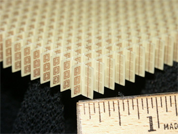
The perfect lens suggestion has triggered a wave of efforts to implement left-hand materials experimentally. (Attempts to find such materials in nature have failed so far.) Most progress in this direction has been achieved using the so-called metamaterials, which are essentially quasi-periodic arrays of specially designed electromagnetic resonators, ideally with high density n >> -3. For example, Fig. 15 shows the metamaterial that was used for the first demonstration of negative refractivity in the microwave region – for ~10-GHz waves.41 It combines straight strips of a metallic film, working as lumped resonators with a large electric dipole moment (and hence strongly coupled to the wave’s electric field E), and several almost-closed film loops (so-called split rings), working as lumped resonators with large magnetic dipole moments, strongly coupled to the field H. The negative refractivity is achieved by designing the resonance frequencies close to each other. More recently, metamaterials with negative refractivity were demonstrated in the optical range as well,42 although to the best of my knowledge, their relatively large absorption still prevents practical applications.
Fig. 7.15. An artificial left-hand material
providing negative refraction at microwave
frequencies ~10 GHz. The original by Jeffrey
D. Wilson (in the public domain) is available
at https://en.wikipedia.org/wiki/Metamaterial.
This progress has stimulated the development of other potential uses of metamaterials (not necessarily the left-handed ones), in particular, designs of nonuniform systems with handcrafted distributions (r, ) and (r, ) that may provide electromagnetic wave propagation along the desired paths, e.g., around a certain region of space, making it virtually invisible for an external observer – so far, within very limited frequency ranges.43
As was mentioned in Sec. 5.5, another way to reach negative values of () is to place a ferromagnetic material into such an external dc magnetic field that the frequency r of the ferromagnetic resonance is somewhat lower than . If thin layers of such a material (e.g., nickel) are interleaved with layers of a non-magnetic good conductor (such as copper), the average value of () of the resulting metamaterial may be positive but substantially below 0. According to Eq. (6.33), the skin-depth s of such a material may be larger than that of the good conductor alone, enforcing a more uniform distribution of the ac current flowing along the layers, and hence making the energy losses lower than in the good conductor alone. This effect may be useful, in particular, for electronic circuit interconnects.44
41 R. Shelby et al., Science 292, 77 (2001); J. Wilson and Z. Schwartz, Appl. Phys. Lett. 86, 021113 (2005).
42 See, e.g., J. Valentine et al., Nature 455, 376 (2008).
43 For a review of such “invisibility cloaks”, see, e.g., B. Wood, Comptes Rendus Physique 10, 379 (2009).
44 See, for example, N. Sato et al., J. Appl. Phys. 111, 07A501 (2012), and references therein.
Chapter 7
Page 29 of 70
EM: Classical Electrodynamics
7.5. Transmission lines: TEM waves
So far, we have analyzed plane electromagnetic waves, implying that their cross-section is infinite – evidently, an unrealistic assumption. The cross-section may be limited, still sustaining wave propagation, using wave transmission lines:45 long, uniform structures made of either good conductors or dielectrics. Let us first discuss the first option, using the following simplifying assumptions: (i) the structure is a cylinder (not necessarily with a round cross-section, see Fig. 16) filled with a usual (right-handed), uniform dielectric material with negligible energy losses ( ” = ” = 0), and (ii) the wave attenuation due to the skin effect is also negligibly low. (As Eq. (78) indicates, for that the characteristic size a of the line’s cross-section has to be much larger than the skin-depth s of its wall material. The energy dissipation effects will be analyzed in Sec. 9 below.)
z
E n
E
z
z
Fig. 7.16. Electric field’s
decomposition in a transmission
y
0
line (in particular, a waveguide).
x
E t
With such exclusion of energy losses, we may look for a particular solution of the macroscopic Maxwell equations in the form of a monochromatic wave traveling along the line:
E(r, t) Re
i( k z
t)
E ( x, y)
z
e
H r
,
( , t) Re
i( k z t)
H ( x, y)
z
e
,
(7.98)
with real kz, where the z-axis is directed along the transmission line – see Fig. 16. Note that this form allows a substantial coordinate dependence of the electric and magnetic field within the plane [ x, y] of the transmission line’s cross-section, as well as nonvanishing longitudinal components Ez and/or Hz of the fields, so the solution (98) is substantially more general than the plane waves discussed above. We will see in a minute that as a result, the parameter kz may be very much different from its plane-wave value (13), k ()1/2, in the same material, at the same frequency.
In order to describe these effects quantitatively, let us decompose the complex amplitudes of the wave’s fields into their longitudinal and transverse components (Fig. 16):46
E E n E
H H n H
,
.
(7.99)
z
z
t
z
z
t
45 Another popular term is the waveguide, but it is typically reserved for the transmission lines with singly-connected cross-sections, to be analyzed in the next section. The first structure for guiding waves was proposed by J. J. Thomson in 1893, and experimentally tested by O. Lodge in 1894.
46 For the notation simplicity, I am dropping index in the complex amplitudes of the field components, and also have dropped the argument in kz and Z, even though these parameters may depend on the wave’s frequency rather substantially – see below.
Chapter 7
Page 30 of 70
EM: Classical Electrodynamics
Plugging Eqs. (98)-(99) into the source-free Maxwell equations (2), and requiring the longitudinal and transverse components to be balanced separately, we get
ik n E i
H
E n
ik n H i
E
H n
z
z
t
t
t
z z ,
z
z
t
t
t
z z ,
E i
H
n ,
H i
E
n ,
(7.100)
t
t
z
z
t
t
z
z
E ik
E ,
H ik
H .
t
t
z
z
t
t
z
z