Applied Computational Fluid Dynamics by Hyoung Woo Oh - HTML preview
Download the book in PDF, ePub, Kindle for a complete version.


Advances in Computational Fluid Dynamics Applied to the Greenhouse Environment
39
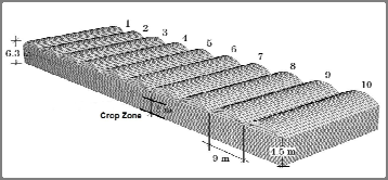
Computational Domain
Fig. 2. Computational mesh generation for a greenhouse (Flores-Velázquez, 2010).
The presence of turbulence in a fluid is indicated by the fluctuating velocity components
and the quantities carried out by the flow, even when the boundary conditions for the
problem under study are kept constant. These fluctuations determine the difference between
laminar flow and turbulent flow (Figure 3). For most situations, ventilation (effect of
temperature, wind or both) measurements and visualization experiments have
demonstrated the turbulent air flow inside and outside the greenhouse. Therefore, the
phenomenon of turbulence must be taken into account (Norton et al. 2007).
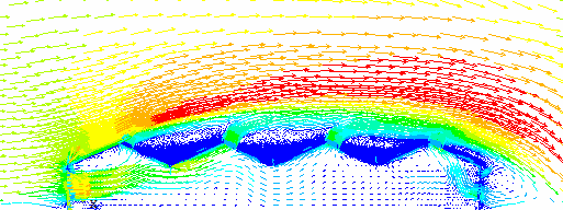
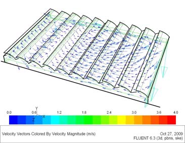
Fig. 3. Velocity vectors on a multi-hood greenhouse of four spans. CFD model considers
anti-insect mesh vents (Rico-García, 2008).


40
Applied Computational Fluid Dynamics
If inertial effects are large enough with respect to viscous effects, then the flow can be
turbulent. Turbulence means that the instantaneous velocity varies at each point of the
flow field. The turbulent nature of the velocity can be explained considering that the rate
consists of the sum of two components, a main component (stable) and a fluctuating
component. Depending on Reynolds number, laminar or turbulent flow can be modeled.
For instance, most turbulence models, such as standard k-ε Model, and Re-Normalized
Group Turbulence Model (RNG), to name a few (Rico-García, 2008).
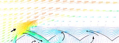
The post-processing stage allows the user to visualize and search for the solution. Figures
contours, vectors and graphs can be obtained from analyzing the solution. It is remarkable
that figures allow us to observe the full distribution of temperature, speed, pressure and
so on the whole flow field (Figure 4).
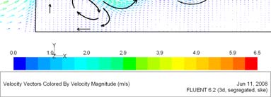
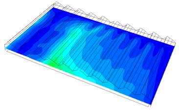
Fig. 4. Wind velocity (m s-1) and temperature (K) representative post processing
characteristics at different greenhouses sceneries (Flores-Velázquez, 2010)
As soon as a CDF model has been tested, the computational greenhouse environment can
become a powerful climate analysis tool. Nowadays, it is possible to visualize, for instance, the wind distribution along the greenhouse when the income windows are up or down, and
also the consequent temperature profiles, among many other possibilities (Figure 5). Even
though, in the last decade research on wind behavior inside the greenhouse has been
enormous, still, as a fundamental part of the greenhouse environment modeling process, it
is necessary to take into consideration the physical verification in order to provide accuracy on the results obtained by numerical simulation (Flores-Velázquez, 2010). Scale models,
water and wind tunnels and direct measurements of the climatic variables are some of the
Advances in Computational Fluid Dynamics Applied to the Greenhouse Environment
41
main options for verification of the CFD models of the greenhouse climate (Flores-
Velázquez, et al., 2011).
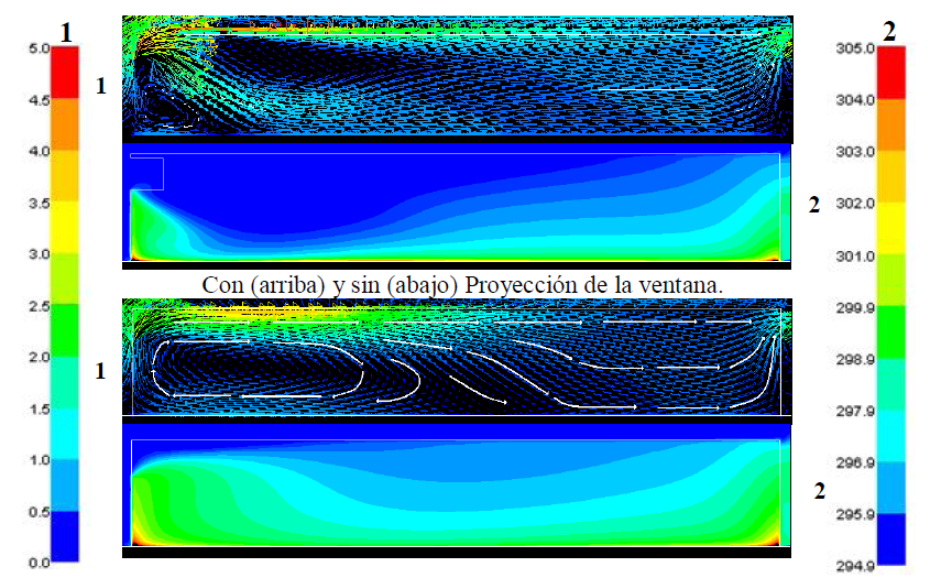
Fig. 5. Comparison of wind speed (m s-1) (1) and profiles of air temperature (K) (2) in the
greenhouse with and without the projection of the rectangular window. Wind speed
exterior 4 m s-1, soil heat flux 315 W m-2 (Flores-Velázquez, 2010).
3. Approaches used in the application of CFD to the greenhouse environment
CFD modeling is used to design facilities that provide suitable climatic conditions for the
crops. According to Sase (2006), within a mild climate, appropriate design and control of
ventilation are required to ensure effective cooling and uniformity of the environment. It is possible to design an optimal greenhouse by calculating its area, volume and vents area as
well as the material properties of the roof (Impron et al. , 2007). Rico-García et al. (2006), comparing two different greenhouses, showed the importance of its geometry and found
that the ventilation rate for a greenhouse with larger vertical roof and windows was better
than a multi-span greenhouse. Omer (2009) describes several designs of low energy
greenhouses. In agreement with Baeza et al. (2008), design changes in the greenhouse, such as size and shape of vents, can improve air movement in the area of crops. Bakker et al.
(2008) investigated energy balance, and determined that the amount of energy used per unit
of output is defined by improvements in energy conversion, environmental control to
reduce energy consumption and efficiency of agricultural production. In a study of outdoor
42
Applied Computational Fluid Dynamics
areas using the turbulence model Reynolds-averaged Navier-Stokes equations (RANS), van
Hoff (2010) found that small geometric modifications can increase the ventilation rate up to 43%. The performance of ventilation in enclosed spaces is affected by the flow of outside air, type of cover, height of the installation and the ventilation opening (Kim et al. , 2010).
Computational parametric studies on greenhouse structures can help to identify design
factors that affect greenhouse ventilation under specific climatic conditions (Romero-Gómez
et al., 2008; Romero-Gómez et al. , 2010; Flores-Velázquez et al., 2008).
3.1 Windward and leeward wind directions
The wind direction outside the greenhouse is an important factor in defining the flow of air and climate inside the greenhouse system. The boundary conditions of wind speed
distribution are deduced from experimental data and wind direction with respect to the
longitudinal axis of the greenhouse, which can range from 0 ° to 90 °. Roy and Boulard
(2005) simulated the impact of wind at 45 ° and 90 °, showing the influence of wind
direction in the air velocity, temperature and humidity distributions inside the greenhouse; a similar result was found by Campen (2003). Rico-García et al. (2006) also showed that a greenhouse with larger vertical roof windows works better with a windward condition,
whereas the multi-span greenhouse works better with a leeward condition. Therefore, wind
direction affects the degree of ventilation. In a experiment carried out by Khaoua et al.
(2006), four different openings of roof vents obtained ventilation rates from 9 to 26.5 air
exchanges per hour for the windward and 3.7 to 12.5 on the leeward wind condition,
respectively, which can maintain acceptable and uniform climate conditions for particular
cases where the wind is perpendicular to the main axis of the greenhouse. Overhead
ventilation to the windward and leeward directions represents a reduction in the ventilation rate by 25% to 45%, compared with only opening to the windward direction (Bournet et al. , 2007). Openings to the windward direction generate the highest rate of ventilation; however, the greatest homogeneity of the temperature and wind speed arises from combining
windward and leeward roof vents (Bournet and Khaoua, 2007).
Kacira et al. (2008) showed that the air temperature inside the greenhouse was higher on the windward side than on the leeward side when roof vents were used. Wind speed had a
linear influence on air exchange rates, while the wind direction did not affect them.
Majdoubi et al. (2009) observed a strong wind air current above a tomato canopy that was fed by a windward side vent and a slow air stream flowing within the tomato canopy space.
The first third of the greenhouse, until the end of the leeward side, was characterized by a combination of wind and buoyancy forces, with warmer and more humid inside air that
was removed through upper roof vents. There may be a conflict between increasing
ventilation and improving uniformity because there is little information on air movement
affecting the cooling efficiency and the uniformity of the environment (Sase, 2006).
According to Rico-García (2008) the relationship between the thermal gradient and
ventilation of gases show