Precalculus: An Investigation of Functions by David Lippman and Melonie Rasmussen - HTML preview
Download the book in PDF, ePub, Kindle for a complete version.
Section 1.3 Rates of Change and Behavior of Graphs 37
F( )
6 − F( )
2 =
6 − 2
2
2
−
62 22
Simplifying
6 − 2
2
2
−
36 4
Combining the numerator terms
4
−16
36
Simplifying further
4
−1 Newtons per centimeter
9
This tells us the magnetic force decreases, on average, by 1/9 Newtons per centimeter
over this interval.
Example 6
Find the average rate of change of g( t)
2
= t + 3 t +1on the interval [ ,
0 a]. Your answer
will be an expression involving a.
Using the average rate of change formula
g( a) − g( )
0
Evaluating the function
a − 0
( 2
a + 3 a + )
1 − (02 + (
3 )
0 + )
1
Simplifying
a − 0
a 2 + a
3 +1−1
Simplifying further, and factoring
a
a( a + )
3
Cancelling the common factor a
a
a + 3
This result tells us the average rate of change between t = 0 and any other point t = a.
For example, on the interval [0, 5], the average rate of change would be 5+3 = 8.
Try it Now
3. Find the average rate of change of f ( x)
3
= x + 2 on the interval [ a, a + h].
38 Chapter 1
Graphical Behavior of Functions
As part of exploring how functions change, it is interesting to explore the graphical
behavior of functions.
Increasing/Decreasing
A function is increasing on an interval if the function values increase as the inputs
increase. More formally, a function is increasing if f(b) > f(a) for any two input values a and b in the interval with b>a. The average rate of change of an increasing function is positive.
A function is decreasing on an interval if the function values decrease as the inputs
increase. More formally, a function is decreasing if f(b) < f(a) for any two input values a and b in the interval with b>a. The average rate of change of a decreasing function is negative.
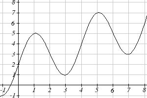
Example 7
Given the function p(t) graphed here, on what
intervals does the function appear to be
increasing?
The function appears to be increasing from t = 1
to t = 3, and from t = 4 on.
In interval notation, we would say the function
appears to be increasing on the interval (1,3) and
the interval ( ,
4 ∞)
Notice in the last example that we used open intervals (intervals that don’t include the
endpoints) since the function is neither increasing nor decreasing at t = 1, 3, or 4.
Local Extrema
A point where a function changes from increasing to decreasing is called a local
maximum.
A point where a function changes from decreasing to increasing is called a local
minimum.
Together, local maxima and minima are called the local extrema, or local extreme
values, of the function.
Section 1.3 Rates of Change and Behavior of Graphs 39
Example 8
Using the cost of gasoline function from the beginning of the section, find an interval on
which the function appears to be decreasing. Estimate any local extrema using the
table.
t
2
3
4
5
6
7
8
9
C(t)
1.47
1.69
1.94
2.30
2.51
2.64
3.01
2.14
It appears that the cost of gas increased from t = 2 to t = 8. It appears the cost of gas
decreased from t = 8 to t = 9, so the function appears to be decreasing on the interval
(8, 9).
Since the function appears to change from increasing to decreasing at t = 8, there is
local maximum at t = 8.
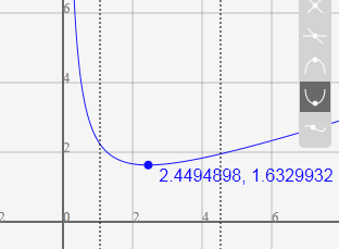
Example 9
Use a graph to estimate the local extrema of the function
2
f ( x)
x
= + . Use these to
x 3
determine the intervals on which the function is increasing.
Using technology to graph the function, it
appears there is a local minimum
somewhere between x = 2 and x =3, and a
symmetric local maximum somewhere
between x = -3 and x = -2.
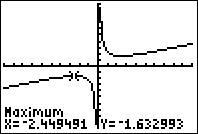
Most graphing calculators and graphing
utilities can estimate the location of
maxima and minima. Below are screen
images from two different technologies,
showing the estimate for the local maximum and minimum.
Based on these estimates, the function is increasing on the intervals (−∞,− .2 )
449 and
(2
,
449
.
∞) . Notice that while we expect the extrema to be symmetric, the two different
technologies agree only up to 4 decimals due to the differing approximation algorithms
used by each.
40 Chapter 1
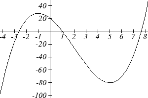
Try it Now
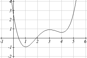
4. Use a graph of the function f ( x)
3
= x − 6 2
x −15 x + 20 to estimate the local extrema
of the function. Use these to determine the intervals on which the function is increasing
and decreasing.
Concavity
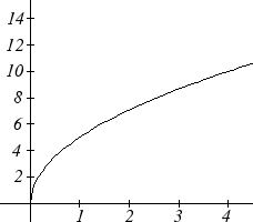
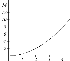
The total sales, in thousands of dollars, for two companies over 4 weeks are shown.
Company A
Company B
As you can see, the sales for each company are increasing, but they are increasing in very
different ways. To describe the difference in behavior, we can investigate how the
average rate of change varies over different intervals. Using tables of values,
Company A
Company B
Week
Sales
Rate of
Week
Sales
Rate of
Change
Change
0
0
0
0
5
0.5
1
5
1
0.5
2.1
1.5
2
7.1
2
2
1.6
2.5
3
8.7
3
4.5
1.3
3.5
4
10
4
8
From the tables, we can see that the rate of change for company A is decreasing, while
the rate of change for company B is increasing.
Section 1.3 Rates of Change and Behavior of Graphs 41
Smaller
Larger
increase
Larger
increase
increase
Smaller
increase
When the rate of change is getting smaller, as with Company A, we say the function is
concave down. When the rate of change is getting larger, as with Company B, we say
the function is concave up.
Concavity
A function is concave up if the rate of change is increasing.
A function is concave down if the rate of change is decreasing.
A point where a function changes from concave up to concave down or vice versa is
called an inflection point.
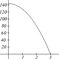
Example 10
An object is thrown from the top of a building. The object’s height in feet above
ground after t seconds is given by the function
2
h( t) = 144 −16 t for 0 ≤ t ≤ 3 . Describe
the concavity of the graph.
Sketching a graph of the function, we can see that the
function is decreasing. We can calculate some rates of
change to explore the behavior
t
h(t)
Rate of
Change
0
144
-16
1
128
-48
2
80
-80
3
0
Notice that the rates of change are becoming more negative, so the rates of change are
decreasing. This means the function is concave down.
42 Chapter 1
Example 11
The value, V, of a car after t years is given in the table below. Is the value increasing or decreasing? Is the function concave up or concave down?
t
0
2
4
6
8
V(t)
28000 24342 21162 18397 15994
Since the values are getting smaller, we can determine that the value is decreasing. We
can compute rates of change to determine concavity.
t
0
2
4
6
8
V(t)
28000
24342
21162
18397
15994
Rate of change
-1829
-1590
-1382.5
-1201.5
Since these values are becoming less negative, the rates of change are increasing, so
this function is concave up.
Try it Now
5. Is the function described in the table below concave up or concave down?
x
0
5
10
15
20
g(x)
10000 9000
7000
4000
0
Graphically, concave down functions bend downwards like a frown, and
concave up function bend upwards like a smile.
Increasing
Decreasing
Concave
Down
Concave
Up
Section 1.3 Rates of Change and Behavior of Graphs 43
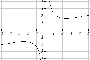
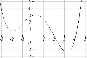
Example 12
Estimate from the graph shown the
intervals on which the function is
concave down and concave up.
On the far left, the graph is decreasing
but concave up, since it is bending
upwards. It begins increasing at x = -2,
but it continues to bend upwards until
about x = -1.
From x = -1 the graph starts to bend
downward, and continues to do so until about x = 2. The graph then begins curving
upwards for the remainder of the graph shown.
From this, we can estimate that the graph is concave up on the intervals (−∞,− )1 and
( ,
2 ∞) , and is concave down on the interval (− ,
1 )
2 . The graph has inflection points at x
= -1 and x = 2.
Try it Now
6. Using the graph from Try it Now 4, f ( x)
3
= x − 6 2
x −15 x + 20, estimate the
intervals on which the function is concave up and concave down.
Behaviors of the Toolkit Functions
We will now return to our toolkit functions and discuss their graphical behavior.
Function
Increasing/Decreasing
Concavity
Constant Function
Neither increasing nor
Neither concave up nor down
f ( x) = c
decreasing
Identity Function
Increasing
Neither concave up nor down
f ( x) = x
Quadratic Function
Increasing on ( ,
0 ∞)
Concave up (−∞,∞)
2
f ( x) = x
Decreasing on (−∞ )
0
,
Minimum at x = 0
Cubic Function
Increasing
Concave down on (−∞ )
0
,
3
f ( x) = x
Concave up on ( ,
0 ∞)
Inflection point at (0,0)
Reciprocal
Decreasing (−∞ 0
, ) ∪ ( ,
0 ∞) Concave down on (−∞ )
0
,
1
f ( x) =
Concave up on ( ,
0 ∞)
x
44 Chapter 1
Function
Increasing/Decreasing
Concavity
Reciprocal squared
Increasing on (−∞ )
0
,
Concave up on (−∞ )
0
, ∪ ( ,
0 ∞)
1
f ( x) =
Decreasing on ( ,
0 ∞)
2
x
Cube Root
Increasing
Concave down on ( ,
0 ∞)
3
f ( x) = x
Concave up on (−∞ )
0
,
Inflection point at (0,0)
Square Root
Increasing on ( ,
0 ∞)
Concave down on ( ,
0 ∞)
f ( x) = x
Absolute Value
Increasing on ( ,
0 ∞)
Neither concave up or down
f ( x) = x
Decreasing on (−∞ )
0
,
Important Topics of This Section
Rate of Change
Average Rate of Change
Calculating Average Rate of Change using Function Notation
Increasing/Decreasing
Local Maxima and Minima (Extrema)
Inflection points
Concavity
Try it Now Answers
−
1.
01
.
3
$
69
.
1
$
32
.
1
$
=
= 0.264 dollars per year.
5 years
5 years
f 9
( ) − f )
1
(
(9−2 9)−(1−2 1) ( )3−(− )
2. Average rate of change =
1
4 1
=
=
= =
9 −1
9 −1
9 −1
8 2
f ( a + h) − f ( a) (( a + h)3 + 2)− ( a 3 + 2) a 3 + a 3 2 h + ah
3 2 + h 3 + 2 − a 3 −
3.
=
=
2 =
( a + h) − a
h
h
2
2
3
3 a h + 3 ah + h
h( 2
2
3 a + 3 ah + h )
2
2
=
= 3 a + 3 ah + h
h
h
4. Based on the graph, the local maximum appears
to occur at (-1, 28), and the local minimum
occurs at (5,-80). The function is increasing
on (−∞,− )
1 ∪ ,
5
( ∞) and decreasing on (− )
5
,
1 .
Section 1.3 Rates of Change and Behavior of Graphs 45
5. Calculating the rates of change, we see the rates of change become more negative, so
the rates of change are decreasing. This function is concave down.
x
0
5
10
15
20
g(x)
10000
9000
7000
4000
0
Rate of change
-1000
-2000
-3000
-4000
6. Looking at the graph, it appears the function is concave down on (−∞, )2 and
concave up on ( ,
2 ∞) .
46 Chapter 1
Section 1.3 Exercises
1. The table below gives the annual sales (in millions of dollars) of a product. What was
the average rate of change of annual sales…
a) Between 2001 and 2002?
b) Between 2001 and 2004?
year 1998 1999 2000 2001 2002 2003 2004 2005 2006
sales 201 219 233 243 249 251 249 243 233
2. The table below gives the population of a town, in thousands. What was the average
rate of change of population…
a) Between 2002 and 2004?
b) Between 2002 and 2006?
year
2000 2001 2002 2003 2004 2005 2006 2007 2008
population 87
84
83
80
77
76
75
78
81
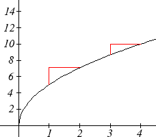
3. Based on the graph shown, estimate the
average rate of change from x = 1 to x = 4.
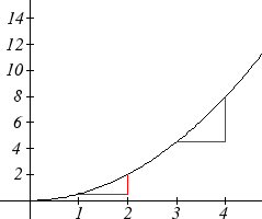
4. Based on the graph shown, estimate the
average rate of change from x = 2 to x = 5.