Parallel Manipulators Towards New Applications by Huapeng Wu - HTML preview
Download the book in PDF, ePub, Kindle for a complete version.
it is a new command, the state of the task is changed to S1 and the status of the task is
changed to indicate that it is executing.
Pick and Place Next Beam
S0 New Command
S1 Hold – Status=Executing
S1 Conditions Good to Move to Pre-Pick Pose
S2 Move to Pre-Pick Pose
S1 Timed out
S0 Hold – Status=Error
S2 Conditions Good to Move to Pick Pose
S3 Move to Pick Pose
S3 Conditions Good to Grasp
S4 Grasp Beam
S4 Conditions Good to Pre-Load Crane
S5 Pre-Load Crane
S5 Conditions Good to Move to Pre-Place Pose
S6 Move to Pre-Place Pose
S6 Conditions Good to Move to Place Pose
S7 Move to Place Pose
S7 Conditions Good to Unload Crane
S8 Unload Crane
S8 Conditions Good to Release
S9 Release Beam
S9 Conditions Good to Move to Post Place Pose
S10 Move to Post Place Pose
S10 At Post Place Pose
S0 Hold - Status=Done
Table 1. State table for the pick and place next beam task.
The next time the above state table is checked (i.e., during the next execution cycle of its
corresponding control module) the new state of the task is S1, and the conditions that must
be met are whether it is acceptable to move RoboCrane to the beam’s pre-pick pose, or
whether enough time has elapsed that something must be wrong. There may be one or more
sub-conditions that must be satisfied in order to determine whether it is acceptable to
proceed, but these can be aggregated into one description in the state table. If the conditions
are met, the state of the task is changed to S2 and the command to move to the pre-pick pose
is sent to a lower-level task. If time has expired, the state of the task is changed to S0 and an
error is reported. Each lower level task that receives an output command reports its status
back to the higher level task that issued the command until it finishes executing or
18
Parallel Manipulators, Towards New Applications
encounters an error. This process continues until all of the commands in the state table have
been executed, at which point the pick and place next beam task is considered completed
and the state of the table is reset to S0. For brevity, only a single timeout condition is shown
in Table 1. In practice, numerous checks of this sort are made throughout the state table.
Once the state tables for all of the tasks identified through the task decomposition process
are completed they are organized into control modules as described next and implemented
in software following the RCS guidelines.
Control Modules: As indicated in the prior RCS description, the commands in the task tree
diagram of Figure 11 are organized into multiple levels. Each level’s tasks may be grouped
together into one or more modules responsible for coordinating and executing the tasks
within it. Some of the critical modules (such as the servo algorithms) run as real-time
processes within the operating system, while other less critical modules (such as long term
path planning) run as non-deterministic processes.
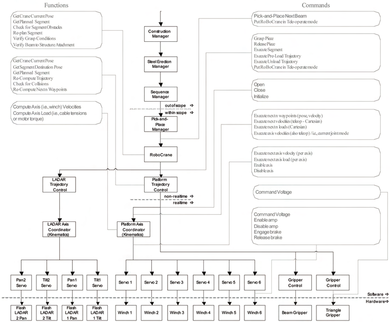
Figure 12 shows the control architecture for the RoboCrane controller. The four levels above
the software/hardware demarcation line in Figure 12 correspond to the four levels of
Figure 11. The tasks have been grouped into the control modules shown. For example, the
bottom level tasks of Figure 11 are grouped into the six “Servo” modules in Figure 12.
Fig. 12. RoboCrane controller architecture diagram.
Control of Cable Robots for Construction Applications
19
Each of these modules are responsible for executing a servo algorithm which accepts the
actual and desired positions (or velocity) of a winch motor as inputs and calculates a
command voltage which maintains the desired position (or velocity). An alternate
configuration would be to group the six servo modules into one.
Figure 12 also shows that the RoboCrane controller is part of a larger control architecture
which includes four higher-level modules. For example, at the level above the RoboCrane
controller would be a Pick-and-Place Manager that would actually command RoboCrane to
perform the pick-and-place operation. The commands sent down by each module to a
lower-level module are shown in the light gray boxes on the right. Some of the functions (or
non-physical tasks) that each module performs are also shown in the light gray boxes on the
left. The control modules above the Pick-and-Place Manager are also included in the figure.
Finally, Figure 12 also includes modules for controlling the 3D imaging systems. These
modules are responsible for coordinating the sensor orientations with the RoboCrane
platform’s motion in order to maintain a desired part of RoboCrane’s environment within
the combined sensors’ field of view.
6. Conclusion
This chapter presented new research developments at NIST in control algorithms and
controller design for parallel robots applied to Construction applications. In particular, this
research focused on the NIST RoboCrane platform for automated placement of construction
components. This work was the first to demonstrate the use of a laser-based site
measurement system for 6 degree-of-freedom tracking of a robotic crane, and presented new
methods for incorporating pose estimation errors in a compensation transform for the NIST
GoMotion controller. Finally, this work presented task decomposition approaches for
analyzing and automating construction crane operations based on a NIST 4D/RCS
approach.
7. References
Albus, J., Huang, H., Messina, E., Murphy, K., Juberts, M., Lacaze, A., Balakirsky, S.,
Shneier, M., Hong, T., & Scott, H. (2002). 4D/RCS Version 2.0: A Reference Model
Architecture for Unmanned Vehicle Systems. National Institute of Standards and
Technology, Gaithersburg, MD, NISTIR 6912.
Albus, J.S., Bostelman, R.V., & Dagalakis, N.G. (1992). The NIST ROBOCRANE, A Robot
Crane. Journal of Robotic Systems, July.
Barbera, T., Albus, J., Messina, E., Schlenoff, C., & Horst, J. (2004). How task analysis can be
used to derive and organize the knowledge for the control of autonomous vehicles.
Robotics and Autonomous Systems 49(1-2), 67-78.
Bostelman, R., Jacoff, A., Dagalakis, N., & Albus, J. (1996). RCS-Based RoboCrane
Integration. Proc. Intelligent Systems: A Semiotic Perspective, Gaithersburg, MD, Oct,
20-23.
Bostelman, R., Shackleford, W., Proctor, F., Albus, J., & Lytle, A. (2002). The Flying Carpet:
A Tool to Improve Ship Repair Efficiency. American Society of Naval Engineers
Symposium, Bremerton, WA, Sept, 10-12.
20
Parallel Manipulators, Towards New Applications
Gazi, V. (2001). The RCS Handbook: Tools for Real-time Control Systems Software
Development. Wiley.
Tsai, L.W. (1999). Robot Analysis: The Mechanics of Serial and Parallel Manipulators. Wiley-
Interscience.
2
Dynamic Parameter Identification for
Parallel Manipulators
Vicente Mata1, Nidal Farhat1, Miguel Díaz-Rodríguez2,
Ángel Valera3 and Álvaro Page4,
Universidad Politécnica de Valencia, Departamento de Mecánica y Materiales Valencia1,
Universidad de los Andes, Facultad de Ingeniería,
Departamento de Tecnología y Diseño Mérida2,
Universidad Politécnica de Valencia, Departamento de Ingeniería
de Sistemas y Automática Valencia3,
Universidad Politécnica de Valencia, Departamento de Física Aplicada Valencia4,
España1,3,4,
Venezuela2
1. Introduction
The information provided by robot manufacturers regarding the dynamic parameters of
robotic systems (the inertial properties of the links and friction parameters at the kinematic
joints) is limited and even nonexistent. For instance, friction parameters are generally not
provided. Thus, it is necessary to develop efficient procedures for their measurement. The
direct measurement of these parameters is not practical since it would imply disassembling
the robot. On the other hand, obtaining these parameters from the CAD models has the
disadvantage that some parts can not be modeled in full detail and parameters that depend
on operational conditions, like friction, can not be determined. For these reasons, parameters
identification has turned out to be a widely accepted technique for determining the dynamic
parameters. This chapter provides an overview of parameters identification processes
applied to parallel manipulators. Practical implementation issues are also considered. In
addition, an approach that considers the identification problem as a nonlinear constrained
optimization problem is presented. Moreover, an evaluation of the accuracy of the solution
of parameters is also addressed.
The importance of inertial and friction parameters lies in their application in most of the
recent literature for advanced model-based control algorithms. The accuracy of dynamic
parameters plays an important role in the precision, performance, stability and robustness of
these control algorithms (Khalil & Dombre, 2002). On the other hand, they are important in
dynamic simulation. It is known that the validation of the direct dynamic problem depends
considerably on the precision of the dynamic parameters of the mechanical system. An
accurately modeled robot permits the substitution of the real mechanical system by a virtual
one thus avoiding the expensive experimental tests used to adjust the operational
parameters for this system (Hiller et al., 2002). Additionally, another important field in
which accurate knowledge of the dynamic parameters is needed is in path planning
22
Parallel Manipulators, Towards New Applications
algorithms that take into account robot dynamics. The predicted forces depend greatly on
the accuracy of the estimated inertial and friction parameters. Hence, inaccurate estimates of
the dynamic parameters may lead to an overloaded robot (dynamically or statically), which
is the case in approximately 50% of industrial robots (Swevers et al., 2002).
Initially, dynamic parameter identification procedures for estimating the dynamic
parameters of open loop mechanical structures were developed in the middles eighties
(Khosla & Kanade, 1985; Atkeson et al., 1986; Olsen & Bekey, 1986; Gautier & Khalil, 1988).
Since then, they have been widely used and several contributions to serial robot dynamics
application control and simulation have been made.
Identification procedures can be classified into two main groups: indirect and direct
approaches. On the one hand, indirect procedures act sequentially in several stops. In each
step, parameters of a different nature (basically friction and some inertial terms) are
identified by means of specifically designed experiments. On the other hand, in the direct
approach, all the parameters are identified in the same stage. A detailed comparison
between the direct and the indirect approaches, applied to a PUMA industrial robot, can be
found in Benimeli et al. (2006). The indirect approach has the disadvantage that errors due
to the noise in the measured data are being accumulated throughout the different stages
(Khalil & Dombre, 2002). Moreover, it is difficult to maintain the working conditions
constant not only throughout these stages, but also within the same one.
For parallel manipulators, the direct approach has been applied (Renaud et al., 1993;
Guegan et al., 2003; Farhat et al., 2008). Meanwhile, the indirect approach has been proposed
(Grotjahn et al., 2004; Abdellatif et al., 2007). However, apart from error accumulation in
each step, the separation of the parameters of a different nature is not straightforward as for
open chain manipulators. Due to the fact that the direct approach allows parameters
identification in one single experiment, removing the accumulation of error between steps,
this chapter will be focus on the direct approach applied to parallel manipulators.
The first part of the chapter deals with conventional direct dynamic parameters
identification processes. Thus, the dynamic model, suitable for identification purposes, is
developed in its linear form with respect to the dynamic parameters. Due to the fact that the
number of parameters is usually greater than the dimension of the equations of motion, an
overdetermined system is developed. This overdetermined system is rank deficient,
therefore it has to be reduced to another equivalent system that only contains independent
columns. These columns correspond to a subset of parameters called the base parameters.
Reduction process can be held symbolically (Khalil & Bennis, 1995) or numerically (Gautier,
1991). For experiment design and in order to reduce the sensitivity of the system to the noise
signal, procedures have been developed for the trajectories to be executed by the
manipulator (Gautier & Khalil, 1992; Swevers et al., 1997). Finally, the dynamic system in its
reduced matrix form is solved for the base parameters using the Least Square Method
(LSM).
The parameters dynamic identification procedure outlined in the previous paragraph has
two main disadvantages: firstly, results could contain non-physically feasible parameters
and secondly, it is also limited to linear friction models. Non-physical feasibility can be
detected by obtaining a base parameters solution that does not have any physical
interpretation when compared with corresponding combinations of the inertial parameters;
masses lower than zero or non positive-definite local inertial matrices (Yoshida & Khalil,
2000). This issue not only affects the stability of some of the advanced model-based control
algorithms, but is also crucial in the dynamic simulation tasks.
Dynamic Parameter Identification for Parallel Manipulators
23
The second part of the chapter will focus on two identification procedures. First, a
procedure based on the parameters identification formulated as a nonlinear constrained
optimization problem is reviewed. This approach allows not only the implementation of
nonlinear friction models to model friction phenomenon at robot joints, but also the
consideration of constraint equations in order to ensure the physical feasibility of the
identified parameters. The second procedure is established upon the accuracy of the
parameter solution, which is called here the identifiability of the parameters . Experiments
will be held on a class of parallel manipulator. The main conclusions and further research
concerning parameters identification for parallel manipulators are presented at the end.
2. Dynamic model
The starting point of the identification process depends on obtaining the dynamic model of
the mechanical structure in its linear form with respect to the inertial and friction
parameters. For this purpose, the dynamic model can be developed basically by two
methods (Kozlowski, 1998); the integral and the differential methods. The integral method is
derived from the energy equation and requires measurements of positions, velocities and
applied forces on the actuated joints. Measurements of accelerations are not required. This
method has been applied on serial manipulators (Gautier & Khalil, 1988; Sheu & Walker,
1989; Khalil et al., 1990; Sheu & Walker, 1991) and extended for parallel manipulators
(Bhattacharya et al., 1997). Olsen and others also used the integral method (Olsen &
Petersen, 2001; Olsen et al., 2002) where they proposed the use of the maximum likelihood
method instead of the conventional Least Squares Method (LSM) in the identification
process.
On the other hand, the differential method takes the advantage of the equations of motion as
a base in the development of the identification process algorithms. As a result, acceleration
appears explicitly and needs to be measured. It is known that the equations of motion can be
constructed implementing various dynamic principles. Models suitable for the identification
process have been developed by means of; the Newton-Euler formulation (Luh et al., 1980;
Atkeson et al., 1986; Olsen & Bekey, 1986; Khosla, 1989), the Lagrange formulation (Ha et al.,
1989; Sheu & Walker, 1991), Jourdain’s principle of Virtual Power (Grotjahn et al., 2004),
Gibbs-Appell equations of motion (Benimeli et al., 2003) and recently (Hardeman et al.,
2006), a finite element based approach along with Jourdain’s principle of Virtual Power was
used to develop an automatic generation of the dynamic models for identification.
In order to study the advantages/disadvantages of the integral and differential methods, a
comparison was carried out. The experiments were held considering a two degrees of
freedom serial manipulator (Prufer et al., 1994). From the results, they concluded that the
differential method has advantages over the integral one. Thus, the differential model is
used here for parameters identification of parallel manipulators.
2.1 Rigid body model
The equation of motion that describes the dynamic behavior of an open chain manipulator
can be obtained by means of Gibbs-Appell equations of motion. For a serial robot (Mata et
al., 2002), the rigid body dynamic model can be written as follows,
24
Parallel Manipulators, Towards New Applications
n ⎧⎛
T
T
⎪ ∂ i ω
⎫
n ⎡
i
⎤
⎞
⎛ r
i
i
i
i
i
i
⎪
∂
⎞
τ =
I
( I
)
m
r
(1)
k
∑ ⎜⎨
⎟ ⋅ ⎡
⋅ ω + ω ×
⋅ ω ⎤
G
i
i
G
i
⎬ +
⎢
G
i
i
i
∑ ⎜
i ⎟ ⋅
⋅
⎥
⎣
⎦
i k
∂ q
q
k
i k ⎢⎜ ∂
⎟
i
Gi
=
⎝
⎪
⎠
=
⎥
⎩
⎪⎭
⎝
k ⎠
⎣
⎦
where τ and q are the generalized forces and accelerations of the joint k, respectively, iω
k
k
i
is the angular acceleration, and i r is the acceleration of the center of gravity, m is the
Gi
i
mass and iI is the inertial tensor of the center of gravity, and the superscript/subscript (i)
Gi
stands for the link number. All of them expressed with respect to the ith local reference
frame. The Denavit-Hartenberg modified convention has been considered for modeling the
system and i = k..n indicates the sum over all links above joint k, including itself.
For dynamic parameters identification, a linear form with respect to dynamic parameters is
necessary. To this end (Atkeson et al., 1986), the linear acceleration of the center of gravity of
the ith body is expressed as a function of the linear acceleration of the link coordinate frame
ith. Moreover, the link inertial tensor is also expressed about the link coordinate frame by
means of parallel axis theorem.
In addition, the following notations are introduced. On the one hand, the cross product
a × b is expressed using the skew symmetric matrix a . Thus, a × b = a ⋅ b where,
⎛ 0
−a
a ⎞
z
y
⎜
⎟
T
a = a
0
−
⎜
a and b = ⎡b
b
b ⎤
z
x ⎟
⎣ x
y
z ⎦
(2)
⎜ a
a
0 ⎟
−
⎝
y
x
⎠
On the other hand, B ⋅ a = â ⋅ B where,
⎛a
a
a
0
0
0 ⎞
x
y
z
⎜
⎟
T
â = ⎜ 0 a
0 a
a
0 and B = ⎡B
B
B
B
B
B ⎤
x
y
z
⎟
⎣ xx
xy
xz
yy
yz
zz ⎦
(3)
⎜ 0 0 a
0 a
a ⎟
⎝
x
y
z ⎠
By doing the above mentioned, upon substituting (2)-(3) in (1) and using some vector
identities, the dynamic model linear with respect to dynamic parameters can be written as
(Mata et al., 2005),
⎧
n
k T
z ⋅ ∑ k
i
R
ηˆ ⋅ i I +
⎪
i
i
i
i
i
i
r
r
m r
r
r
m
k : R
k
i ⎣ i
i
(
η −
OkOi
i
Oi )
⎫
⎡
⋅
+
⋅
⎤
i
OiGi
OkOi
Oi
i ⎦
⎪
⎪
i k
⎪
=
τ =
(4)
k
⎨
⎬
⎪
z ∑n
k T
k R (
i
i
i
m
r
m r
k : P
k
i
i
Oi
i
i
Oi ,Gi )
⎪
⋅
⋅
⋅
+ η ⋅
⎪
⎪
⎩
i =k
⎭
where i ˆη = ( i
i
i
ˆω + ω ˆω y iη = ( i i
i
ω ω + ω .
i
i
i