LabVIEW Graphical Programming by Serhat Beyenir - HTML preview
Download the book in PDF, ePub, Kindle for a complete version.
Chapter 5
Plotting Data
5.1 Waveform Charts1
The ✇❛✈❡❢♦r♠ ❝❤❛rt is a numeric indicator that displays one or more plots. The ✇❛✈❡❢♦r♠ ❝❤❛rt is located on the ❈♦♥tr♦❧s
●r❛♣❤ ■♥❞✐❝❛t♦rs palette. ❲❛✈❡❢♦r♠ ❝❤❛rts can display single or multiple plots. Fig-
ure 5.1 shows the elements of a multiplot waveform chart. Two plots are displayed: ❘❛✇ ❉❛t❛ and ❘✉♥♥✐♥❣
❆✈❣.
Figure 5.1
Charts use three different modes to scroll data, as shown in the Figure 5.2. Right-click the chart and select
❆❞✈❛♥❝❡❞ ❯♣❞❛t❡ ▼♦❞❡ from the shortcut menu. Select ❙tr✐♣ ❈❤❛rt, ❙❝♦♣❡ ❈❤❛rt, or ❙✇❡❡♣ ❈❤❛rt . The
default mode is ❙tr✐♣ ❈❤❛rt.
Figure 5.2
A str✐♣ ❝❤❛rt shows running data continuously scrolling from left to right across the chart. A s❝♦♣❡
❝❤❛rt shows one item of data, such as a pulse or wave, scrolling partway across the chart from left to the 1This content is available online at <http://cnx.org/content/m12233/1.2/>.
Available for free at Connexions <http://cnx.org/content/col11408/1.1>
87
88
CHAPTER 5. PLOTTING DATA
right. A s✇❡❡♣ ❝❤❛rt is similar to an EKG display. A s✇❡❡♣ ❝❤❛rt works similarly to a scope except it shows the older data on the right and the newer data on the left separated by a vertical line. The s❝♦♣❡
❝❤❛rt and s✇❡❡♣ ❝❤❛rt have retracing displays similar to an oscilloscope. Because there is less overhead in retracing a plot, the s❝♦♣❡ ❝❤❛rt and the s✇❡❡♣ ❝❤❛rt display plots significantly faster than the str✐♣
❝❤❛rt.
5.1.1 Wiring Charts
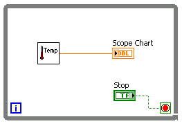
You can wire a s❝❛❧❛r ♦✉t♣✉t directly to a ✇❛✈❡❢♦r♠ ❝❤❛rt. The data type in the ✇❛✈❡❢♦r♠ ❝❤❛rt in
Figure 5.3 terminal matches the input data type.
Figure 5.3
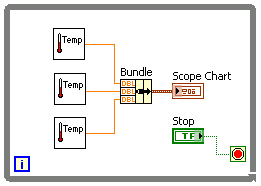
❲❛✈❡❢♦r♠ ❝❤❛rts can display multiple plots. Bundle multiple plots together using the ❇✉♥❞❧❡ function located on the ❈❧✉st❡r palette. In Figure 5.4, the ❇✉♥❞❧❡ function bundles the outputs of the three VIs to plot on the waveform chart.
Figure 5.4
The ✇❛✈❡❢♦r♠ ❝❤❛rt terminal changes to match the output of the ❇✉♥❞❧❡ function. To add more plots,
use the P♦s✐t✐♦♥✐♥❣ tool to resize the ❇✉♥❞❧❡ function.
Available for free at Connexions <http://cnx.org/content/col11408/1.1>

89
5.2 Temperature Monitor VI2
Exercise 5.2.1
Complete the following steps to build a VI that measures temperature and displays it on a wave-
form chart.
5.2.1 Front Panel
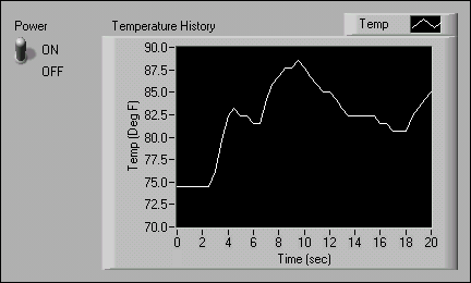
1. Open a blank VI and build the front panel shown in Figure 5.5.
Figure 5.5
a. Place the vertical toggle switch, located on the ❈♦♥tr♦❧s
❇✉tt♦♥s ✫ ❙✇✐t❝❤❡s
palette, on the front panel. Label this switch P♦✇❡r. You use the switch to stop the
acquisition.
b. Place a ✇❛✈❡❢♦r♠ ❝❤❛rt, located on the ❈♦♥tr♦❧s
●r❛♣❤ ■♥❞✐❝❛t♦rs palette, on the
front panel. Label the chart ❚❡♠♣❡r❛t✉r❡ ❍✐st♦r②. The ✇❛✈❡❢♦r♠ ❝❤❛rt displays the
temperature in real time.
c.
The ✇❛✈❡❢♦r♠ ❝❤❛rt ❧❡❣❡♥❞ labels the plot P❧♦t ✵. Use the ▲❛❜❡❧✐♥❣ tool to
triple-click P❧♦t ✵ in the chart legend, and change the label to ❚❡♠♣.
d. The temperature sensor measures room temperature. Use the ▲❛❜❡❧✐♥❣ tool to double-
click 10.0 in the y-axis and type 90 to rescale the chart. Leave the x-axis in its default
state.
e. Change −10.0 in the y-axis to 70.
f. Label the y-axis ❚❡♠♣ ✭❉❡❣ ❋✮ and the x-axis ❚✐♠❡ ✭s❡❝✮.
5.2.2 Block Diagram
1. Select ❲✐♥❞♦✇
❙❤♦✇ ❇❧♦❝❦ ❉✐❛❣r❛♠ to display the block diagram.
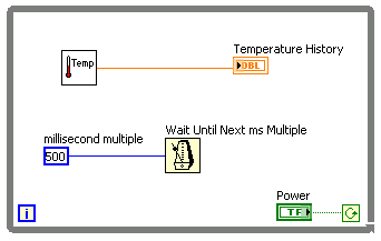
2. Enclose the two terminals in a While Loop, as shown in the block diagram (Figure 5.6).
2This content is available online at <http://cnx.org/content/m12234/1.2/>.
Available for free at Connexions <http://cnx.org/content/col11408/1.1>


90
CHAPTER 5. PLOTTING DATA
Figure 5.6
3. Right-click the ❝♦♥❞✐t✐♦♥❛❧ terminal and select ❈♦♥t✐♥✉❡ ✐❢ ❚r✉❡.
4. Wire the objects as shown in Figure 5.6.
a.
Place the ❚❤❡r♠♦♠❡t❡r VI on the block diagram.
Select ❋✉♥❝t✐♦♥s
❆❧❧
❋✉♥❝t✐♦♥s ❙❡❧❡❝t ❛ ❱■
and
navigate
to
❈✿\❊①❡r❝✐s❡s\▲❛❜❱■❊❲ ❇❛s✐❝s
■\❚❤❡r♠♦♠❡t❡r✳✈✐✳ This subVI returns one temperature measurement from the
temperature sensor.
NOTE: Use the ✭❉❡♠♦✮ ❚❤❡r♠♦♠❡t❡r VI if you do not have a DAQ device available.
b.
Place
the
❲❛✐t ❯♥t✐❧ ◆❡①t ♠s ▼✉❧t✐♣❧❡ function,
located
on
the
❋✉♥❝t✐♦♥s ❆❧❧ ❋✉♥❝t✐♦♥s ❚✐♠❡ ✫ ❉✐❛❧♦❣ palette, on the block diagram.
c.
Right-click the ♠✐❧❧✐s❡❝♦♥❞ ♠✉❧t✐♣❧❡ input of the ❲❛✐t ❯♥t✐❧ ◆❡①t ♠s
▼✉❧t✐♣❧❡ function, select ❈r❡❛t❡ ❈♦♥st❛♥t from the shortcut menu, type 500, and
press the <❊♥t❡r> key. The numeric constant specifies a wait of 500ms so the loop
executes once every half-second.
NOTE: To measure temperature in Celsius, wire a Boolean ❚r✉❡ constant located on the
❋✉♥❝t✐♦♥s ❆r✐t❤♠❡t✐❝ ✫ ❈♦♠♣❛r✐s♦♥ ❊①♣r❡ss ❇♦♦❧❡❛♥ palette to the ❚❡♠♣ ❙❝❛❧❡
input of the ❚❤❡r♠♦♠❡t❡r VI. Change the scales on charts and graphs in subsequent
exercises to a range of 20 to 32 instead of 70 to 90.
5. Save the VI as ❚❡♠♣❡r❛t✉r❡ ▼♦♥✐t♦r✳✈✐ in the ❈✿\❊①❡r❝✐s❡s\▲❛❜❱■❊❲ ❇❛s✐❝s ■ directory.
5.2.3 Run the VI
1. Display the front panel by clicking it or by selecting ❲✐♥❞♦✇
❙❤♦✇ ❋r♦♥t P❛♥❡❧.
2. Use the ❖♣❡r❛t✐♥❣ tool to click the vertical toggle switch and turn it to the ❖◆ position.
3. Run the VI. The subdiagram within the ❲❤✐❧❡ ▲♦♦♣ border executes until the specified con-
dition is ❚r✉❡. For example, while the switch is on (❚r✉❡), the ❚❤❡r♠♦♠❡t❡r VI takes and
returns a new measurement and displays it on the ✇❛✈❡❢♦r♠ ❝❤❛rt.
4. Click the vertical toggle switch to stop the acquisition. The condition is ❋❛❧s❡, and the loop
stops executing.
Available for free at Connexions <http://cnx.org/content/col11408/1.1>
91
5.2.4 Front Panel
1. Format and customize the x- and y-scales of the waveform chart.
a. Right-click the chart and select Pr♦♣❡rt✐❡s from the shortcut menu to display the ❈❤❛rt
Pr♦♣❡rt✐❡s dialog box.
b. Click the ❋♦r♠❛t ❛♥❞ Pr❡❝✐s✐♦♥ tab. Select ❉❡❣ ❋ ✭❨✲❛①✐s✮ in the top pull-down
menu. Set the ❉✐❣✐ts ♦❢ ♣r❡❝✐s✐♦♥ to 1.
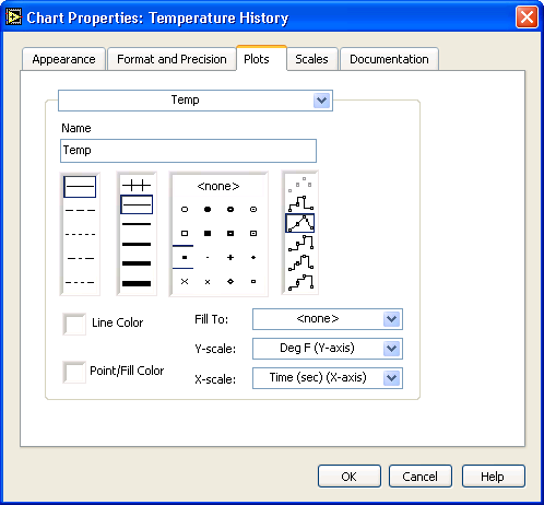
c. Click the P❧♦ts tab and select different styles for the y-axis, as shown in Figure 5.7.
Figure 5.7
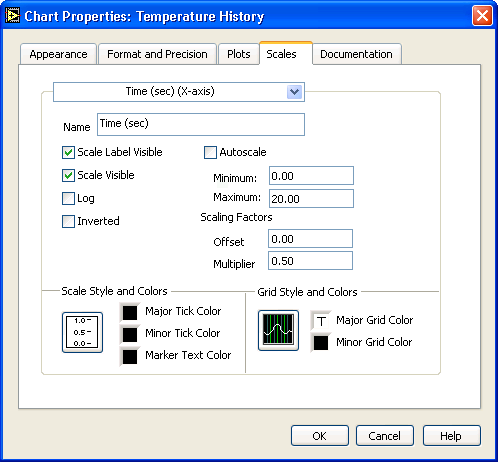
d. Select the ❙❝❛❧❡s tab and select the ❚✐♠❡ ✭s❡❝✮ ✭❳✲❛①✐s✮ in the top pull-down menu.
Set the scale options as shown in Figure 5.8. Set the ▼✉❧t✐♣❧✐❡r to 0.50 to account for
the ✺✵✵ ♠s ❲❛✐t function.
Available for free at Connexions <http://cnx.org/content/col11408/1.1>
92
CHAPTER 5. PLOTTING DATA
Figure 5.8
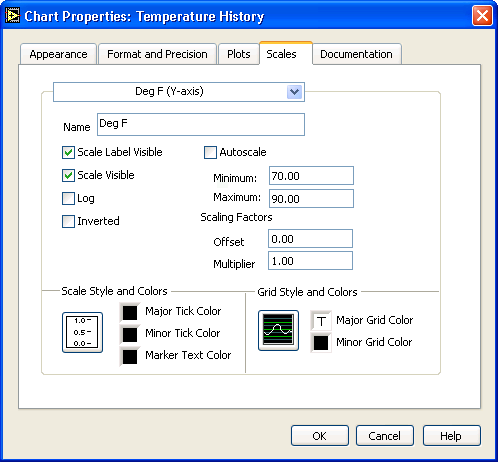
e. In the ❙❝❛❧❡s tab, select the ❉❡❣ ❋ ✭❨✲❛①✐s✮ in the top pull-down menu. Set the scale
options as shown in Figure 5.9.
Available for free at Connexions <http://cnx.org/content/col11408/1.1>

93
Figure 5.9
f. Click the ❖❑ button to close the dialog box when finished.
2. Right-click the ✇❛✈❡❢♦r♠ ❝❤❛rt and select ❉❛t❛ ❖♣❡r❛t✐♦♥s
❈❧❡❛r ❈❤❛rt from the short-
cut menu to clear the display buffer and reset the ✇❛✈❡❢♦r♠ ❝❤❛rt.
TIP: When a VI is running, you can select ❈❧❡❛r ❈❤❛rt from the shortcut menu.
3. Each time you run the VI, you first must turn on the vertical toggle switch and then click the
❘✉♥ button due to the current mechanical action of the switch. Modify the mechanical action
of the vertical toggle switch so temperature is plotted on the graph each time you run the VI,
without having to first set the toggle switch.
a. Stop the VI if it is running.
b. Use the ❖♣❡r❛t✐♥❣ tool to click the vertical toggle switch and turn it to the ❖◆ position.
c. Right-click the switch and select ❉❛t❛ ❖♣❡r❛t✐♦♥s
▼❛❦❡ ❈✉rr❡♥t ❱❛❧✉❡ ❉❡❢❛✉❧t
from the shortcut menu. This sets the ❖◆ position as the default value.
d.
Right-click the switch and select ▼❡❝❤❛♥✐❝❛❧ ❆❝t✐♦♥
▲❛t❝❤ ❲❤❡♥ Pr❡ss❡❞
from the shortcut menu. This setting changes the control value when you click it and
retains the new value until the VI reads it once. At this point the control reverts to its
default value, even if you keep pressing the mouse button. This action is similar to a
circuit breaker and is useful for stopping ❲❤✐❧❡ ▲♦♦♣s or for getting the VI to perform
an action only once each time you set the control.
5.2.5 Run the VI
1. Run the VI.
Available for free at Connexions <http://cnx.org/content/col11408/1.1>

94
CHAPTER 5. PLOTTING DATA
2. Use the ❖♣❡r❛t✐♥❣ tool to click the vertical switch to stop the acquisition. The switch changes
to the ❖❋❋ position and changes back to ❖◆ after the ❝♦♥❞✐t✐♦♥❛❧ terminal reads the value.
3. Save the VI. You will use this VI in the Temperature Running Average (Section 5.3) VI.
5.3 Temperature Running Average VI3
Exercise 5.3.1
Complete the following steps to modify the ❚❡♠♣❡r❛t✉r❡ ▼♦♥✐t♦r VI to average the last three
temperature measurements and display the average on a ✇❛✈❡❢♦r♠ ❝❤❛rt.
5.3.1 Front Panel
1. Open the Temperature Monitor (Section 5.2) VI.
2. Select ❋✐❧❡
❙❛✈❡ ❆s and rename the VI ❚❡♠♣❡r❛t✉r❡ ❘✉♥♥✐♥❣ ❆✈❡r❛❣❡✳✈✐ in the
❈✿\❊①❡r❝✐s❡s\▲❛❜❱■❊❲ ❇❛s✐❝s ■ directory.
5.3.2 Block Diagram
1. Display the block diagram.
2. Right-click the right or left border of the ❲❤✐❧❡ ▲♦♦♣ and select ❆❞❞ ❙❤✐❢t ❘❡❣✐st❡r from
the shortcut menu to create a s❤✐❢t r❡❣✐st❡r.
3. Right-click the left terminal of the s❤✐❢t r❡❣✐st❡r and select ❆❞❞ ❊❧❡♠❡♥t from the shortcut
menu to add an element to the s❤✐❢t r❡❣✐st❡r.
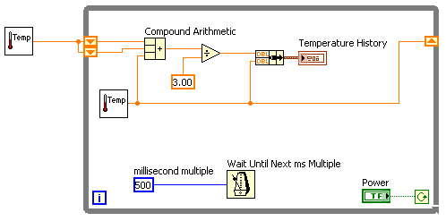
4. Modify the block diagram as in Figure 5.10.
Figure 5.10
a.
Press the <❈tr❧> key while you click the ❚❤❡r♠♦♠❡t❡r VI and drag it outside
the ❲❤✐❧❡ ▲♦♦♣ to create a copy of the subVI. The ❚❤❡r♠♦♠❡t❡r VI returns one tempera-
3This content is available online at <http://cnx.org/content/m12235/1.2/>.
Available for free at Connexions <http://cnx.org/content/col11408/1.1>


95
ture measurement from the temperature sensor and initializes the left s❤✐❢t r❡❣✐st❡rs
before the loop starts.
b.
Place
the
❈♦♠♣♦✉♥❞ ❆r✐t❤♠❡t✐❝
function,
located
on
the
❋✉♥❝t✐♦♥s ❆r✐t❤♠❡t✐❝ ✫ ❈♦♠♣❛r✐s♦♥ ❊①♣r❡ss ◆✉♠❡r✐❝ palette, on the block
diagram.
This function returns the sum of the current temperature and the two
previous temperature readings. Use the P♦s✐t✐♦♥✐♥❣ tool to resize the function to have
three left terminals.
c.
Place the ❉✐✈✐❞❡ function,
located on the ❋✉♥❝t✐♦♥s
❆r✐t❤♠❡t✐❝ ✫
❈♦♠♣❛r✐s♦♥ ❊①♣r❡ss ◆✉♠❡r✐❝ palette, on the block diagram. This function re-
turns the average of the last three temperature readings.
d.
Right-click the ② terminal of the ❉✐✈✐❞❡ function, select ❈r❡❛t❡
❈♦♥st❛♥t, type
3, and press the <❊♥t❡r> key.
5.3.3 Run the VI
1. Run the VI. During each iteration of the ❲❤✐❧❡ ▲♦♦♣, the ❚❤❡r♠♦♠❡t❡r VI takes one temper-
ature measurement. The VI adds this value to the last two measurements stored in the left
terminals of the s❤✐❢t r❡❣✐st❡r. The VI divides the result by three to find the average of
the three measurements, the current measurement plus the previous two. The VI displays
the average on the ✇❛✈❡❢♦r♠ ❝❤❛rt. Notice that the VI initializes the s❤✐❢t r❡❣✐st❡r with
a temperature measurement.
5.3.4 Block Diagram
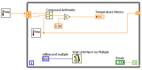
1. Modify the block diagram as shown in Figure 5.11.
Figure 5.11
a.
Place the ❇✉♥❞❧❡ function, located on the ❋✉♥❝t✐♦♥s
❆❧❧ ❋✉♥❝t✐♦♥s ❈❧✉st❡r
palette, on the block diagram. This function bundles the average and current tempera-
ture for plotting on the ✇❛✈❡❢♦r♠ ❝❤❛rt.
Available for free at Connexions <http://cnx.org/content/col11408/1.1>

96
CHAPTER 5. PLOTTING DATA
2. Save the VI. You will use this VI later in the course.
5.3.5 Run the VI
1. Run the VI. The VI displays two plots on the ✇❛✈❡❢♦r♠ ❝❤❛rt. The plots are overlaid. That
is, they share the same vertical scale.
2. If time permits, complete the optional steps. Otherwise, close the VI.
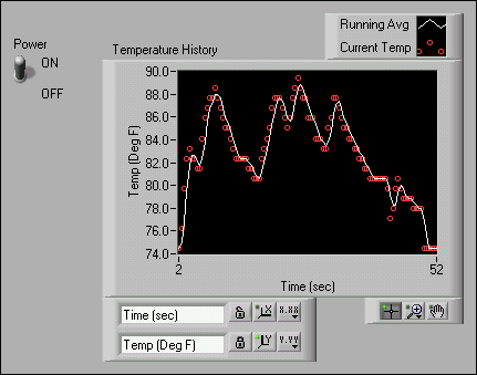
5.3.6 Optional
Customize the waveform chart as shown in Figure 5.12. You can display a plot legend, a scale
legend, a graph palette, a digital display, and a scrollbar. By default, a ✇❛✈❡❢♦r♠ ❝❤❛rt displays
the plot legend.
Figure 5.12
1. Customize the y-axis.
a.
Use the ▲❛❜❡❧✐♥❣ tool to double-click 70.0 in the y-axis, type 75.0, and press the
<❊♥t❡r> key.
b. b - Use the ▲❛❜❡❧✐♥❣ tool to double-click the second number from the bottom on the
y-axis, type 80.0, and press the <❊♥t❡r> key. This number determines the numerical
spacing of the y-axis divisions. For example, if the number above 75.0 is 77.5, it indicates
a y-axis division of 2.5, changing the 77.5 to 80.0 reformats the y-axis to multiples of 5.0
(75.0, 80.0, 85.0, and so on).
NOTE: The ✇❛✈❡❢♦r♠ ❝❤❛rt size has a direct effect on the display of axis scales. Increase the
✇❛✈❡❢♦r♠ ❝❤❛rt size if you encounter problems while customizing the axis.
Available for free at Connexions <http://cnx.org/content/col11408/1.1>
97
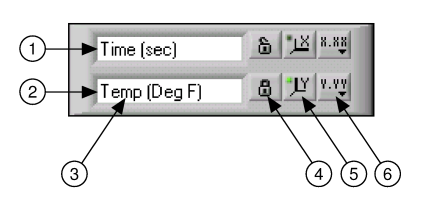
2. Right-click the waveform chart and select ❱✐s✐❜❧❡ ■t❡♠s
❙❝❛❧❡ ▲❡❣❡♥❞ from the shortcut
menu to display the scale legend, as shown in Figure 5.13. You can place the scale legend
anywhere on the front panel.
Figure 5.13: 1. X-axis, 2. Y-axis, 3. Scale Labels, 4. Scale Lock Button, 5. Autoscale Button, 6. Scale Format Button
3. Use the scale legend to customize each axis.
a. Make sure the ▲♦❝❦ ❆✉t♦s❝❛❧❡ button appears locked and the ❆✉t♦s❝❛❧❡ LED is green
so the y-axis adjusts the minimum and maximum values to fit the data in the chart.
b. Click the ❙❝❛❧❡ ❋♦r♠❛t button to change the format, precision, mapping mode, scale
visibility, and grid options for each axis.
4. Use the plot legend to customize the plots.
a. Use the P♦s✐t✐♦♥✐♥❣ tool to resize the plot legend to include two plots.
b. Use the ▲❛❜❡❧✐♥❣ tool to change ❚❡♠♣ to ❘✉♥♥✐♥❣ ❆✈❣ and to change P❧♦t ✶ to ❈✉rr❡♥t
❚❡♠♣. If the text does not fit, use the Positioning tool to resize the plot legend.
c. Right-click the plot in the plot legend to set the line and point styles and the color of the
plot background or traces.
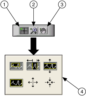
5. Right-click the ✇❛✈❡❢♦r♠ ❝❤❛rt and select ❱✐s✐❜❧❡ ■t❡♠s
●r❛♣❤ P❛❧❡tt❡ from the short-
cut menu to display the graph palette, as shown in Figure 5.14. You can place the graph
palette anywhere on the front panel.
Figure 5.14: 1. Cursor Movement Tool, 2. Zoom Button, 3. Panning Tool, 4. Zoom Pull-down Menu Use the ❩♦♦♠ button on the graph palette to zoom in or out of sections of the chart or the
whole chart. Use the P❛♥♥✐♥❣ tool to pick up the plot and move it around on the display.
Use the ❈✉rs♦r ▼♦✈❡♠❡♥t tool to move the cursor on the graph.
6. Run the VI. While the VI runs, use the buttons in the scale legend and graph palette to modify
the ✇❛✈❡❢♦r♠ ❝❤❛rt.
NOTE:
If you modify the axis labels, the display might become larger than the maximum
size that the VI can correctly present.
7. Use the ❖♣❡r❛t✐♥❣ tool to click the P♦✇❡r switch and stop the VI.
8. Save and close the VI.
Available for free at Connexions <http://cnx.org/content/col11408/1.1>
98
CHAPTER 5. PLOTTING DATA
5.4 Waveform and XY Graphs4
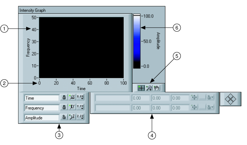
VIs with graphs usually collect the data in an array and then plot the data to the graph. Figure 5.15 shows the elements of a graph.
Figure 5.15
The graphs located on the ❈♦♥tr♦❧s
●r❛♣❤ ■♥❞✐❝❛t♦rs palette include the ✇❛✈❡❢♦r♠ ❣r❛♣❤ and ❳❨
❣r❛♣❤. The ✇❛✈❡❢♦r♠ ❣r❛♣❤ plots only single-valued functions, as in y = f (x), with points evenly distributed along the x-axis, such as acquired time-varying waveforms. ❳❨ ❣r❛♣❤s display any set of points, evenly sampled or not.
Resize the plot legend to display multiple plots. Use multiple plots to save space on the front panel and to make comparisons between plots. ❳❨ and ✇❛✈❡❢♦r♠ ❣r❛♣❤s automatically adapt to multiple plots.
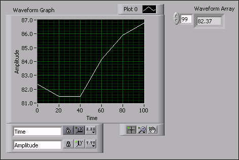
5.4.1 Single Plot Waveform Graphs
The ✇❛✈❡❢♦r♠ ❣r❛♣❤ accepts a single array of values and interprets the data as points on the graph and increments the x index by one starting at x = 0. The graph also accepts a cluster of an initial x value, a
∆ (x), and an array of y data. Refer to the ❲❛✈❡❢♦r♠ ●r❛♣❤ VI in the ◆■ ❊①❛♠♣❧❡ ❋✐♥❞❡r for examples of the data types that single-plot ✇❛✈❡❢♦r♠ ❣r❛♣❤s accept.
5.4.2 Multiplot Waveform Graphs
A multiplot ✇❛✈❡❢♦r♠ ❣r❛♣❤ accepts a 2D array of values, where each row of the array is a single plot. The graph interprets the data as points on the graph and increments the x index by one, starting at x = 0. Wire a 2D array data type to the graph, right-click the graph, and select ❚r❛♥s♣♦s❡ ❆rr❛② from the shortcut menu to handle each column of the array as a plot. Refer to the ✭❨✮ ▼✉❧t✐ P❧♦t ✶ ❣r❛♣❤ in the ❲❛✈❡❢♦r♠ ●r❛♣❤
VI in the ◆■ ❊①❛♠♣❧❡ ❋✐♥❞❡r for an example of a graph that accepts this data type.
A multiplot ✇❛✈❡❢♦r♠ ❣r❛♣❤ also accepts a cluster of an x value, a ∆ (x) value, and a 2D array of y data.
The graph interprets the y data as points on the graph and increments the x index by ∆ (x), starting at x = 0.
Refer to the ✭❳♦✱ ❞❳✱ ❨✮ ▼✉❧t✐ P❧♦t ✸ ❣r❛♣❤ in the ❲❛✈❡❢♦r♠ ●r❛♣❤ VI in the ◆■ ❊①❛♠♣❧❡ ❋✐♥❞❡r for
an example of a graph that accepts this data type.
A multiplot ✇❛✈❡❢♦r♠ ❣r❛♣❤ accepts a cluster of an initial x value, a ∆ (x) value, and an array that contains clusters. Each cluster contains a point array that contains the y data. You use the ❇✉♥❞❧❡ function to bundle the arrays into clusters, and you use the ❇✉✐❧❞ ❆rr❛② function to build the resulting clusters into an array. You also can use the ❇✉✐❧❞ ❈❧✉st❡r Array, which creates arrays of clusters that contain inputs you specify. Refer to the ✭❳♦✱ ❞❳✱ ❨✮ ▼✉❧t✐ P❧♦t ✷ graph in the ❲❛✈❡❢♦r♠ ●r❛♣❤ VI in the ◆■ ❊①❛♠♣❧❡
❋✐♥❞❡r for an example of a graph that accepts this data type.
4This content is available online at <http://cnx.org/content/m12236/1.1/>.
Available for free at Connexions <http://cnx.org/content/col11408/1.1>
99
5.4.3 Single Plot XY Graphs
The s✐♥❣❧❡✲♣❧♦t ❳❨ ❣r❛♣❤ accepts a cluster that contains an x array and a y array. The ❳❨ ❣r❛♣❤ also accepts an array of points, where a point is a cluster that contains an x value and a y value. Refer to the ❳❨
●r❛♣❤ VI in the ◆■ ❊①❛♠♣❧❡ ❋✐♥❞❡r for an example of single-plot ❳❨ ❣r❛♣❤ data types.
5.4.4 Multiplot XY Graphs
The multiplot ❳❨ ❣r❛♣❤ accepts an array of plots, where a plot is a cluster that contains an x array and a y array. The multiplot ❳❨ ❣r❛♣❤ also accepts an array of clusters of plots, where a plot is an array of poin