ECE 454 and ECE 554 Supplemental reading by Don Johnson, et al - HTML preview
Download the book in PDF, ePub for a complete version.
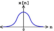
The unit sample.
Examination of a discrete-time signal's plot, like that of the cosine signal shown in Figure 2.9,
reveals that all signals consist of a sequence of delayed and scaled unit samples. Because the value
of a sequence at each integer m is denoted by s( m) and the unit sample delayed to occur at m is
written δ( n− m) , we can decompose any signal as a sum of unit samples delayed to the appropriate
location and scaled by the signal value.
()
This kind of decomposition is unique to discrete-time signals, and will prove useful subsequently.
Unit Step
The unit sample in discrete-time is well-defined at the origin, as opposed to the situation with
analog signals.
()
Symbolic Signals
An interesting aspect of discrete-time signals is that their values do not need to be real numbers.
We do have real-valued discrete-time signals like the sinusoid, but we also have signals that
denote the sequence of characters typed on the keyboard. Such characters certainly aren't real
numbers, and as a collection of possible signal values, they have little mathematical structure
other than that they are members of a set. More formally, each element of the symbolic-valued
signal s( n) takes on one of the values { a 1, …, aK} which comprise the alphabet A . This technical terminology does not mean we restrict symbols to being members of the English or Greek
alphabet. They could represent keyboard characters, bytes (8-bit quantities), integers that convey
daily temperature. Whether controlled by software or not, discrete-time systems are ultimately
constructed from digital circuits, which consist entirely of analog circuit elements. Furthermore,
the transmission and reception of discrete-time signals, like e-mail, is accomplished with analog
signals and systems. Understanding how discrete-time and analog signals and systems intertwine
is perhaps the main goal of this course.
Discrete-Time Systems
Discrete-time systems can act on discrete-time signals in ways similar to those found in analog
signals and systems. Because of the role of software in discrete-time systems, many more
different systems can be envisioned and "constructed" with programs than can be with analog
signals. In fact, a special class of analog signals can be converted into discrete-time signals,
processed with software, and converted back into an analog signal, all without the incursion of
error. For such signals, systems can be easily produced in software, with equivalent analog
realizations difficult, if not impossible, to design.
2.6. Systems in the Time-Domain*
A discrete-time signal s( n) is delayed by n 0 samples when we write s( n− n 0) , with n 0>0 .
Choosing n 0 to be negative advances the signal along the integers. As opposed to analog delays,
discrete-time delays can only be integer valued. In the frequency domain, delaying a signal
corresponds to a linear phase shift of the signal's discrete-time Fourier transform:
( s( n− n 0) ↔ ⅇ–( ⅈ 2 πfn 0) S( ⅇⅈ 2 πf)) .
Linear discrete-time systems have the superposition property.
(2.1)
Superposition
S( a 1 x 1( n)+ a 2 x 2( n))= a 1 S( x 1( n))+ a 2 S( x 2( n)) A discrete-time system is called shift-invariant (analogous to time-invariant analog systems) if delaying the input delays the corresponding output.
(2.2)
Shift-Invariant
If S( x( n))= y( n) , Then S( x( n− n 0))= y( n− n 0) We use the term shift-invariant to emphasize that delays can only have integer values in discrete-time, while in analog signals, delays can be arbitrarily valued.
We want to concentrate on systems that are both linear and shift-invariant. It will be these that
allow us the full power of frequency-domain analysis and implementations. Because we have no
physical constraints in "constructing" such systems, we need only a mathematical specification. In
analog systems, the differential equation specifies the input-output relationship in the time-
domain. The corresponding discrete-time specification is the difference equation.
(2.3)
The Difference Equation
y( n)= a 1 y( n−1)+ …+ apy( n− p)+ b 0 x( n)+ b 1 x( n−1)+ …+ bqx( n− q) Here, the output signal y( n) is related to its past values y( n− l) , l={1, …, p} , and to the current and past values of the input signal x( n) . The system's characteristics are determined by the
choices for the number of coefficients p and q and the coefficients' values { a 1, …, ap} and
{ b 0, b 1, …, bq} .
There is an asymmetry in the coefficients: where is a 0 ? This coefficient would multiply the
y( n) term in the difference equation. We have essentially divided the equation by it, which does not change the input-output relationship. We have thus created the convention that a 0 is
always one.
As opposed to differential equations, which only provide an implicit description of a system (we
must somehow solve the differential equation), difference equations provide an explicit way of
computing the output for any input. We simply express the difference equation by a program that
calculates each output from the previous output values, and the current and previous inputs.
2.7. Autocorrelation of Random Processes*
Before diving into a more complex statistical analysis of random signals and processes, let us quickly review the idea of correlation. Recall that the correlation of two signals or variables is the expected value of the product of those two variables. Since our focus will be to discover more


about a random process, a collection of random signals, then imagine us dealing with two samples
of a random process, where each sample is taken at a different point in time. Also recall that the
key property of these random processes is that they are now functions of time; imagine them as a
collection of signals. The expected value of the product of these two variables (or samples) will now depend on how quickly they change in regards to time. For example, if the two variables are
taken from almost the same time period, then we should expect them to have a high correlation.
We will now look at a correlation function that relates a pair of random variables from the same
process to the time separations between them, where the argument to this correlation function will
be the time difference. For the correlation of signals from two different random process, look at
the crosscorrelation function.
Autocorrelation Function
The first of these correlation functions we will discuss is the autocorrelation, where each of the
random variables we will deal with come from the same random process.
Definition: Autocorrelation
the expected value of the product of a random variable or signal realization with a time-shifted
version of itself
With a simple calculation and analysis of the autocorrelation function, we can discover a few
important characteristics about our random process. These include:
1. How quickly our random signal or processes changes with respect to the time function
2. Whether our process has a periodic component and what the expected frequency might be
As was mentioned above, the autocorrelation function is simply the expected value of a product.
Assume we have a pair of random variables from the same process, X 1= X( t 1) and X 2= X( t 2) , then the autocorrelation is often written as
()
The above equation is valid for stationary and nonstationary random processes. For stationary
processes, we can generalize this expression a little further. Given a wide-sense stationary
processes, it can be proven that the expected values from our random process will be independent
of the origin of our time function. Therefore, we can say that our autocorrelation function will
depend on the time difference and not some absolute time. For this discussion, we will let
τ= t 2− t 1 , and thus we generalize our autocorrelation expression as
()


for the continuous-time case. In most DSP course we will be more interested in dealing with real
signal sequences, and thus we will want to look at the discrete-time case of the autocorrelation
function. The formula below will prove to be more common and useful than Equation:
()
And again we can generalize the notation for our autocorrelation function as
()
Properties of Autocorrelation
Below we will look at several properties of the autocorrelation function that hold for stationary
random processes.
Autocorrelation is an even function for τ R xx( τ)= R xx(– τ)
The mean-square value can be found by evaluating the autocorrelation where τ=0 , which gives
us
The autocorrelation function will have its largest value when τ=0 . This value can appear again,
for example in a periodic function at the values of the equivalent periodic points, but will never
be exceeded. R xx(0)≥| R xx( τ)|
If we take the autocorrelation of a period function, then R xx( τ) will also be periodic with the
same frequency.
Estimating the Autocorrleation with Time-Averaging
Sometimes the whole random process is not available to us. In these cases, we would still like to
be able to find out some of the characteristics of the stationary random process, even if we just
have part of one sample function. In order to do this we can estimate the autocorrelation from a
given interval, 0 to T seconds, of the sample function.
()
However, a lot of times we will not have sufficient information to build a complete continuous-
time function of one of our random signals for the above analysis. If this is the case, we can treat
the information we do know about the function as a discrete signal and use the discrete-time
formula for estimating the autocorrelation.


()
Examples
Below we will look at a variety of examples that use the autocorrelation function. We will begin
with a simple example dealing with Gaussian White Noise (GWN) and a few basic statistical
properties that will prove very useful in these and future calculations.
Example 2.11.
We will let x[ n] represent our GWN. For this problem, it is important to remember the
following fact about the mean of a GWN function: E[ x[ n]]=0
Figure 2.11.
Gaussian density function. By examination, can easily see that the above statement is true - the mean equals zero.
Along with being zero-mean, recall that GWN is always independent. With these two facts,
we are now ready to do the short calculations required to find the autocorrelation.
R xx[ n, n+ m]= E[ x[ n] x[ n+ m]] Since the function, x[ n] , is independent, then we can take the product of the individual expected values of both functions.
R xx[ n, n+ m]= E[ x[ n]] E[ x[ n+ m]] Now, looking at the above equation we see that we can break it up further into two conditions: one when m and n are equal and one when they are not equal.
When they are equal we can combine the expected values. We are left with the following
piecewise function to solve:
We can now solve the two parts of the above
equation. The first equation is easy to solve as we have already stated that the expected value
of x[ n] will be zero. For the second part, you should recall from statistics that the expected
value of the square of a function is equal to the variance. Thus we get the following results for
the autocorrelation:
Or in a more concise way, we can represent the results as
R xx[ n, n+ m]= σ 2 δ[ m]
2.8. DIGITAL CORRELATION*


Convolution is very useful and powerful concept. It appears quite frequently in DSP discussion. It
is begun with a rather twisted definition (folding before shifting), but it then becomes the
representation of linear systems, and is linked to the Fourier transform and the z-transform.
As for convolution, correlation is defined for both analog and digital signals. Correlation of two
signals measure the degree of their similarity. But correlation of a signal with itself also has
meaning and application. The strength of convolution lies in the fact that if applies to signals as
well as systems, whereas correlation only applies to signals. Correlation is used in many areas
such as radar, geophysics, data communications, and, especially, random processes.
Cross-correlation and auto-correlation
Cross-correlation, or correlation for short, between two discrete-time signals x(n) and v(n),
assumed real-valued, is defined as
()
or equivalently
()
Notice that correlation at index n is the summation of the product of one signal and other signal
shifted.
When the signals x(n) and v(n) are interchanged, we get
()
or equivalently
()
Thus
()
Rxv ( m)= Rxv (− m)
This result shows that one correlation is the flipped version (mirror-imaged) of the other, but
otherwise contains the same information.
The evalution of correlation is similar to that of convolution expect no signal flipping is need,
hence the computing steps are slide (shift) – multiply – add. The method of sequence (vector),
as for the convolution ( section ), is one of the possible ways.


Example 2.12.
Find the cross-correlation of the following signals x( n)=[ 2, 5, 2, 4 ] v( n)=[ 2, −3, 1 ] The
figures in bold face are samples at origin.
Solution
First we choose the shorter sequence, in this case v(n), to be shifted, and the longer sequence, x(n),
to stay stationary. Next the evaluate the correlation at m = 0 (no shifting yet), then the correlation
at m = 1, 2, 3 … (shifting v(n) to the right) until v(n) has gone past x(n) completely. Next, we
evaluate the correlation at = -1, -2, -3 … (shifting v(n) to the left) until v(n) has gone past x(n)
completely. At each value of m, we do the multiplication and summing. The evaluation is
arranged as follows. Remember to align the values of x(n) and v(n) at origin at be beginning.
Final result :
Rxv ( m)=[ 2, −1, −9, 8, −8, 8 ]
Example 2.13.
Given two signals
Compute the cross-corelation.
Solution
The cross-correlation is
The summation is divided into two ranges of of m depending on the shifting direction of v(n) with
respect to x(n).


For m < 0, v(n) is shifted to the left of x(n), the summation lower limit is n = 0 :
Where the formula of infinite geometric serics ( Equation ) has been used. Since m < 0, we can write
For m≥0 , v(n) is shifted to the right, the summation lower limit is n = m :
Let’s make a change of variable k = n – m to get
Where the formula finite geometric serics ( Equation ) has been used. Since m 0, we can write On combining the two parts, the overall cross-correlation results
Auto-correlation
Auto-correlation of a signal x(n) is the cross-correlation with itself :
()
or equivalently
()
At m = 0 (no shifting yet) the auto-correlation is maximum because the signal superimposes
completely with itself. The correlation decreases as m increases in both directions.


The auto-correlation is an even symmetric function of m :
()
Rxx ( m)= Rxx (− m)
Example 2.14.
Find the expression for the auto-correlation of the signal given in Example 2.8.2 x( n)= anu( n)
Solution
We have
Since
iseven symmetric we need to compute only the
for m 0 then generalize the result
for the correlation.
For m≥0
Make a change of varible k = n – m as in previous example :
, ∣ a∣2<1
Above result is for m≥0 . Now for all m we just write ∣ m∣ for m because of the even symmetry of
the auto-correlation. So
Correlation and data communication
Consider a digital signal x(n) transmitted to the far end of the communication channel. It reaches
the receiver n 0 samples later, becoming x(n - n 0), and it is also added with random noise z(n).
Thus the total signal at the receiver is
y( n)= x( n−1)+ z( n)
Now let’s look at the cross-correlation betwwen y(n) and x(n) :


<