ECE 454 and ECE 554 Supplemental reading by Don Johnson, et al - HTML preview
Download the book in PDF, ePub for a complete version.
<m:math><m:ci>&omega</m:ci></m:math>
Signal
It is sometimes useful to describe an arbitrary signal, or an input/output relationship. In such
cases, it is recommended that f be used to represent a generic signal. For an input/output
relationship, use x as an arbitrary input signal and y as the arbitrary output signal. When writing
out the signal as a function of some variable, such as time, it can be represented as x( t) for
continuous-time signals and as x[ n] for discrete-time signals.
Example 2.3. MathML Mark-Up
For a continuous-time signal, x( t) :
<m:math>
<m:apply>
<m:ci type="function">x</m:ci>
<m:ci>t</m:ci>
</m:apply>
</m:math>
For a discrete-time signal, x[ n] :
<m:math>
<m:apply>
<m:ci type="fn" class="discrete">x</m:ci>
<m:ci>n</m:ci>
</m:apply>
</m:math>
Special Signals
There are several signals used often enough to merit special attention. They are presented here.
Impulse
The impulse, or Dirac-Delta function, should be presented as δ( t) in continuous-time and as δ[ n] in discrete-time.
The impulse is a signal which could be given a definitionURL, which in conjunction with
csymbol would allow us to facilitate the coding of the mathematical expression.
Example 2.4. MathML Mark-Up
<!-- Continuous Time -->
<m:math>
<m:apply>
<m:ci type='fn'>δ</m:ci>
<m:ci>t</m:ci>
</m:apply>
</m:math>
<!-- Discrete Time -->
<m:math>
<m:apply>
<m:ci type='fn' class='discrete'>δ</m:ci>
<m:ci>n</m:ci>
</m:apply>
</m:math>
Unit Step
The unit step should be presented as u( t) in continuous-time and as u[ n] in discrete-time. These
functions will be marked-up in MathML the same as the delta function above; however, rather
than the δ symbol you will use u .
The unit step is a signal which could be given a definitionURL, which in conjunction with
csymbol would allow us to facilitate the coding of the mathematical expression.


Sinc
The sinc function should be represented as
()
The sinc function is a signal which could be given a definitionURL, which in conjunction with
csymbol would allow us to facilitate the coding of the mathematical expression. This has not
happened yet so, for now, we are using the following markup:
Example 2.5. MathML Mark-Up
<m:math>
<m:apply>
<m:ci type='fn'>sinc</m:ci>
<m:ci>x</m:ci>
</m:apply>
</m:math>
Norm
The norm of a vector or function should be represented as ∥x∥ For instance, the Euclidean norm
(sometimes called the L2-norm) of a vector should be given by
()
The norm operator has been given a csymbol but are still working on the rendering of it. The
correct code can be seen below and was used to mark-up the first instance of the norm of x in
the above paragraph.
Example 2.6. MathML Mark-Up
<m:math>

<m:apply>
<m:csymbol definitionURL='http://cnx.rice.edu/cd/cnxmath.ocd#norm'/>
<m:ci type='vector'>x</m:ci>
</m:apply>
</m:math>
Convolution
Convolution is given by and should be displayed as
()
The convolution operator is defined by a csymbol which can be used through the following
CNXML/MathML code.
Example 2.7. MathML Mark-Up
<m:math>
<m:apply>
<m:csymbol definitionURL='http://cnx.rice.edu/cd/cnxmath.ocd#convolve'/>
<m:ci>f</m:ci>
<m:ci>g</m:ci>
</m:apply>
</m:math>
Circular Convolution
Standard notation for circular convolution, or periodic convolution, uses a circled asterick, ⊛ , between two variables or functions. See the equation below as an example:
y( t)=( f( t) ⊛ g( t)) Although a csymbol for regular convolution exists, there is still not a proper mathematical way to mark-up circular convolution. Until a csymbol or MathML tag is created, we
advise using the following code:

<m:math>
<m:apply>
<m:ci><m:mo>⊛</m:mo></m:ci>
<m:ci>f</m:ci>
<m:ci>g</m:ci>
</m:apply>
</m:math>
Twiddle Factor
The Twiddle factor should be displayed as
()
The twiddle factor could be given a definitionURL, which in conjunction with, probably given
by <twiddle/>.
Example 2.8. MathML Mark-Up
<m:math>
<m:ci>
<m:msub>
<m:mi>W</m:mi>
<m:mi>N</m:mi>
</m:msub>
</m:ci>
</m:math>
Fourier Transform
Although the concept of the Fourier transform is well-known, there are variations in the precise definition of the transform. It is recommended that the following notation be used for the Fourier
transform. Which particular transform is used (discrete Fourier transform, continuous-time
Fourier series, discrete-time Fourier transform, etc) should be apparent from context (these all
assume that x is the function to be transformed):
CTFT: X( Ω)
<m:math>
<m:apply>
<m:ci type='fn'>X</m:ci>
<m:ci>Ω</m:ci>
</m:apply
</m:math>
DTFT: X( ω)
<m:math>
<m:apply>
<m:ci type='fn'>X</m:ci>
<m:ci>ω</m:ci>
</m:apply
</m:math>
DFT: X[ n]
<m:math>
<m:apply>
<m:ci type='fn' class='discrete'>X</m:ci>
<m:ci>n</m:ci>
</m:apply
</m:math>
The Fourier operator ℱ[·] could be given a definitionURL, which in conjunction with
csymbol would allow us to facilitate the coding of the mathematical expression.


CTFT
There are a few ways of describing the Fourier transform. The recommended notation for the
transform is given as:
()
Laplace Transform
The Laplace transform is defined as
()
where s= σ+ ⅈΩ is the complex frequency. The unilateral Laplace transform, or one-side Laplace,
is defined exactly the same but the lowlimit of the integral is 0 rather than –∞ .
The Laplace operator [·] could be given a definitionURL, which in conjunction with
csymbol would allow us to facilitate the coding of the mathematical expression.
<m:math>
<m:apply>
<m:ci type="fn" class="discrete">ℒ</m:ci>
<m:apply>
<m:ci type="fn">x</m:ci>
<m:ci>t</m:ci>
</m:apply>
</m:apply>
</m:math>
z-transform
The (unilateral) z-transform is given by
()

where z= σ+ ⅈω is complex in general.
The z-transform operator Z[·] could be given a definitionURL, which in conjunction with
csymbol would allow us to facilitate the coding of the mathematical expression.
<m:math>
<m:apply>
<m:ci type="fn" class="discrete">Z</m:ci>
<m:apply>
<m:ci type="fn" class="discrete">f</m:ci>
<m:ci>n</m:ci>
</m:apply>
</m:apply>
</m:math>
Complex Numbers
As is common in electrical engineering, it is recommended that the complex number ⅈ be used to denote
. Use <m:imaginaryi/> to mark-up all instances of the imaginary number, ⅈ . Use
the following notation and code for operations dealing with complex numbers.
The modulus of a complex number z will be represented as | z| .
<m:math>
<m:apply>
<m:abs/>
<m:ci>z</m:ci>
</m:apply>
</m:math>
The argument of complex number z will be rendered as ∠( z) using the arg tag in MathML.
The standard notation in electrical engineering often denotes the argument simply as ∠ z , but
this does not utilize the arg tag. See the codeblock below to see how both of these
representations should be implemented:

<!-- Using arg tag in MathML -->
<m:math>
<m:apply>
<m:arg/>
<m:ci>z</m:ci>
</m:apply>
</m:math
<!-- Using presentation MathML to render standard EE notation -->
<m:math>
<m:ci>
<m:mrow>
<m:mo>∠</m:mo>
<m:mi>z</m:mi>
</m:mrow>
</m:ci>
</m:math>
The conjugate of a complex number z will be represented as z* . The default rendering for the
conjugate tag in MathML is . The first notation is more common to electrical engineers
and can be rendered using the following MathML code:
<m:math>
<m:ci>
<m:msup>
<m:mi>z</m:mi>
<m:mo>*</m:mo>
</m:msup>
</m:ci>
</m:math>
The abs tag in MathML content can be used to display the modulus with the default
rendering. However, the arg and the conjugate tags' default rendering is not the
recommended rendering. The correct rendering will be implemented using an XSL
transformation. The Connexions project has already implemented the use of j for the
imaginary unit in its stylesheets.

Inner Product
The inner product (or scalar product) of two vectors is given by
()
The MathML code used to denote an inner product follows. Note that this code is for a more
simplified expression, only dealing with x and y rather than a subscripted variable as seen in the
equation above.
<m:math>
<m:apply>
<m:scalarproduct/>
<m:ci type="vector">x</m:ci>
<m:ci type="vector">y</m:ci>
</m:apply>
</m:math>
2.2. Discrete-Time Systems in the Time-Domain*
A discrete-time signal s( n) is delayed by n 0 samples when we write s( n− n 0) , with n 0>0 .
Choosing n 0 to be negative advances the signal along the integers. As opposed to analog delays,
discrete-time delays can only be integer valued. In the frequency domain, delaying a signal
corresponds to a linear phase shift of the signal's discrete-time Fourier transform:
( s( n− n 0) ↔ ⅇ–( ⅈ 2 πfn 0) S( ⅇⅈ 2 πf)) .
Linear discrete-time systems have the superposition property.
()
S( a 1 x 1( n)+ a 2 x 2( n))= a 1 S( x 1( n))+ a 2 S( x 2( n)) A discrete-time system is called shift-invariant (analogous to time-invariant analog systems) if delaying the input delays the corresponding output. If S( x( n))= y( n) , then a shift-invariant system has the property
()
S( x( n− n 0))= y( n− n 0)
We use the term shift-invariant to emphasize that delays can only have integer values in discrete-
time, while in analog signals, delays can be arbitrarily valued.
We want to concentrate on systems that are both linear and shift-invariant. It will be these that
allow us the full power of frequency-domain analysis and implementations. Because we have no
physical constraints in "constructing" such systems, we need only a mathematical specification. In
analog systems, the differential equation specifies the input-output relationship in the time-
domain. The corresponding discrete-time specification is the difference equation.
()
y( n)= a 1 y( n−1)+ …+ apy( n− p)+ b 0 x( n)+ b 1 x( n−1)+ …+ bqx( n− q) Here, the output signal y( n) is related to its past values y( n− l) , l={1, …, p} , and to the current and past values of the input signal x( n) . The system's characteristics are determined by the
choices for the number of coefficients p and q and the coefficients' values { a 1, …, ap} and
{ b 0, b 1, …, bq} .
There is an asymmetry in the coefficients: where is a 0 ? This coefficient would multiply the
y( n) term in Equation. We have essentially divided the equation by it, which does not change the input-output relationship. We have thus created the convention that a 0 is always one.
As opposed to differential equations, which only provide an implicit description of a system (we
must somehow solve the differential equation), difference equations provide an explicit way of
computing the output for any input. We simply express the difference equation by a program that
calculates each output from the previous output values, and the current and previous inputs.
Difference equations are usually expressed in software with for loops. A MATLAB program that
would compute the first 1000 values of the output has the form
for n=1:1000
y(n) = sum(a.*y(n-1:-1:n-p)) + sum(b.*x(n:-1:n-q));
end
An important detail emerges when we consider making this program work; in fact, as written it
has (at least) two bugs. What input and output values enter into the computation of y(1) ? We need
values for y(0) , y(-1) , ..., values we have not yet computed. To compute them, we would need
more previous values of the output, which we have not yet computed. To compute these values, we
would need even earlier values, ad infinitum. The way out of this predicament is to specify the
system's initial conditions: we must provide the p output values that occurred before the input
started. These values can be arbitrary, but the choice does impact how the system responds to a
given input. One choice gives rise to a linear system: Make the initial conditions zero. The reason
lies in the definition of a linear system: The only way that the output to a sum of signals can be the sum of the individual outputs occurs when the initial conditions in each case are zero.
The initial condition issue resolves making sense of the difference equation for inputs that start at
some index. However, the program will not work because of a programming, not conceptual,
error. What is it? How can it be "fixed?"
The indices can be negative, and this condition is not allowed in MATLAB. To fix it, we must
start the signals later in the array.
Example 2.9.
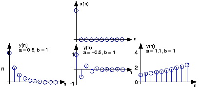
Let's consider the simple system having p=1 and q=0 .
()
y( n)= ay( n−1)+ bx( n)
To compute the output at some index, this difference equation says we need to know what the
previous output y( n−1) and what the input signal is at that moment of time. In more detail,
let's compute this system's output to a unit-sample input: x( n)= δ( n) . Because the input is zero
for negative indices, we start by trying to compute the output at n=0 .
()
y(0)= ay(-1)+ b
What is the value of y(–1) ? Because we have used an input that is zero for all negative
indices, it is reasonable to assume that the output is also zero. Certainly, the difference
equation would not describe a linear system if the input that is zero for all time did not produce a zero output. With this assumption, y(-1)=0 , leaving y(0)= b . For n>0 , the input
unit-sample is zero, which leaves us with the difference equation y( n)= ay( n−1) , n>0 . We can envision how the filter responds to this input by making a table.
()
y( n)= ay( n−1)+ bδ( n)
Table 2.2.
n
x( n) y( n)
–1 0
0
0
1
b
1
0
ba
2
0
ba 2
:
0
:
n
0
ban
Coefficient values determine how the output behaves. The parameter b can be any value, and
serves as a gain. The effect of the parameter a is more complicated (Table 2.2). If it equals
zero, the output simply equals the input times the gain b. For all non-zero values of a, the
output lasts forever; such systems are said to be IIR (Infinite Impulse Response). The reason
for this terminology is that the unit sample also known as the impulse (especially in analog