Honors Chemistry Lab Fall by Mary McHale - HTML preview
Download the book in PDF, ePub, Kindle for a complete version.
By building the models of various molecules during this lab, you will be able to better understand molecular symmetry and isomers. Building models is not difficult; however, the chemical
principles involved are very important and you may find some surprises in how atoms can be fit
together.
Finally, in Part 4, you will be applying your knowledge of VSEPR (Valence Shell Electron Pair
Repulsion) Theory in order to determine the geometry of several different molecules. VSEPR
theory is useful in helping to determine how atoms will orient themselves in molecules. Basically, the idea is that the arrangement adopted by a molecule will be the one in which the repulsions
among the various electron domains are minimized. The two kinds of electron domains are
bonding (electron pair shared by two atoms) and non-bonding (electron density centralized on one atom) pairs of electrons.
Experimental Procedure
For Parts 1 & 2: You and your lab partner are to work with one other lab group in preparing these models (no more than 3 - 4 students). Your TA will assign each group a certain set of molecules to make and answer questions pertaining to those molecules. Each group will then present their
answers to the class. These models will need to be completed and answers determined within 30
minutes so that we can continue to Parts 3 & 4 as soon as possible.
For Parts 1-4, the work should be divided among the group members. Be sure to discuss the
questions and answers among yourselves, but put your own conclusions on the Report Form.
1. Symmetry Elements
Using the Molecular Framework models, make models of the following compounds:
1. CH4
2. CH3Cl
3. CH2Cl2
4. CHCl3
5. CH2ClF
6. CHBrClF
7. BF3
8. BF2Cl
9. PH3
10. PH2Cl
Choose a color to represent each atom. For example, make all C atoms black, all H atoms white,
etc.
Once the models are created, look for symmetry elements that may be present. Ask yourselves the following questions:
Does the molecule contain a mirror plane (σ)? In other words, is there a plane within the molecule which results in one half being a mirror image of the other half?
Does the molecule contain a two-fold rotation axis (C2)? Remember from the Introduction
that the subscript indicates the degrees of rotation necessary to reach a configuration that is indistinguishable from the original one. In this case, the rotation will be 180o.
Does the molecule contain any higher-order rotation axes?
C3 – rotation by 120o
C4 – rotation by 90o
C∞ (infinity rotation axis) – rotation of any amount will result in an indistinguishable orientation
Does the molecule have an inversion center (i)?
Determine which of these symmetry elements are present in your assigned molecules. All of the
columns of the table on the report form should be filled out. If you have any difficulty
determining whether such symmetry elements are present in the molecules you are assigned, your
TA can provide examples of each symmetry element.
Extra credit points can be earned by indicating in the table how many of each symmetry element
are present for each molecule (i.e. How many mirror planes are present?).
2.Mirror Images
Using the model kits, build models which are the mirror images of the models you were assigned
to build (b, c, d, e, f, g, h, i and j) in Part 1. With the two mirror images in hand, try to place the models on top of one another, atom for atom.
If you can do this, the model and its mirror image are superimposable mirror images of one another. If not, the molecule and its mirror image form nonsuperimposable mirror images.
Nonsuperimposable mirror images are also known as enantiomers.
For each compound, decide whether the mirror image is superimposable or nonsuperimposable.
Can you make a generalization about when to expect molecules to have nonsuperimposable mirror
images?
3.Isomers
In this exercise you will build models of compounds which are structural and/or geometrical
isomers of one another.
Make the following models:
A. Structural Isomers
1. Make a model(s) of C2H5Cl. How many different structural isomers are possible?
2. Make a model(s) of C3H7Cl. How many different structural isomers are possible?
3. Make a model(s) of C3H6Cl2. How many different structural isomers are possible?
B. Geometrical Isomers
1. Make a model(s) of C2H3Cl. How many different structural and geometrical isomers are
possible?
2. Make a model(s) of C2H2Cl2. How many different structural and geometrical isomers are
possible?
3. Make a model(s) of cyclobutane (C4H8). HINT: cyclo = ring of C atoms
4. Now make dichlorocyclobutane (C4H6Cl2) by replacing two H atoms on cyclopropane with Cl
atoms. How many different structural and geometrical isomers are possible for
dichlorocyclobutane? You may wish to make a couple of cyclobutane molecules so that you
can compare the structures. Do any of the isomers have nonsuperimposable mirror images?
C. Aromatic Ring Compounds
1. Make a model of benzene, C6H6. Even though your model will contain alternating double and
single bonds, remember that in the real molecules of benzene all the C-C bonds are equivalent.
What symmetry elements does benzene possess?
2. Make a model(s) of chlorobenzene, C6H5Cl. How many different structural and geometrical
isomers are possible?
3. Make a model(s) of dichlorobenzene, C6H4Cl2. How many different structural and geometrical
isomers are possible?
4. Make a model(s) of trichlorobenzene, C6H3Cl3. How many different structural and geometrical isomers are possible?
4. Hypervalent Structures
Hypervalent compounds are those that have more than an octet of electrons around them. Such compounds are formed commonly with the heavier main group elements such as Si, Ge, Sn, Pb, P,
As, Sb, Bi, S, Se, Te, etc. but rarely with C, N or O. Refer to the rules for Electron Domain theory in order to assign Lewis structures to the following molecules. Describe possible isomeric forms and the bond angles between the atoms. How many lone pairs of electrons are present on the
central atom of each molecule, if any? (** Your book will be very useful in aiding you with these structures **)
1. PF5
2. PF3Cl2
3. SF4
4. XeF2
5. BrF3
5. BrF3
Solutions
Chapter 4. Beer's Law and Data Analysis
Beer’s Law and Data Analysis
Objectives
Learn or review typical data analysis procedures – plotting data with excel, performing linear
regression analysis, etc.
Explore the concepts and applications of spectrophotometry
Grading
Pre-lab (10%)
Lab Report Form – including plot (80%)
TA points + Pop Quiz (10%)
Before coming to lab…
Read the lab instructions
Print out the lab instructions and report form.
Complete the pre-lab, due at the beginning of the lab
Introduction
When describing chemical compounds, scientists rely on their chemical and physical properties.
In lab, we might observe that a metal reacts violently with water, that a reactant is liquid at room temperature, or that a powder is yellow. Chemical and physical properties can be used
qualitatively to identify a material or to predict its behavior, or quantitatively to determine how much of that material is present in a solution. In this lab, we will develop a scheme to determine the concentration of copper sulfate in aqueous solution using spectrophotometry.
To start, we will consider light and its interaction with matter. Chemicals exhibit a diverse range of colors, especially when they contain transition metal ions. In order for a compound to have
color, it must absorb visible light. Visible light consists of electromagnetic radiation with
wavelengths ranging from approximately 400 nm to 700 nm, a small section of the
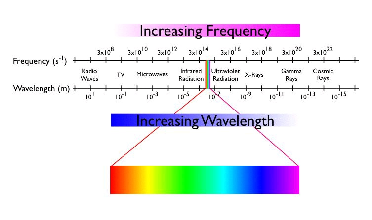
electromagnetic radiation spectrum shown below.
Light is characterized by its frequency ( ν), the number of times the crest of the wave passes some point in space per second, or by its wavelength ( λ), the distance between two successive crests.
These two quantities are related by the speed of light, a fundamental constant: λν= c=3×10⁸m/s.
Planck related the frequency of light to its energy (E) according to E=hν, where h is Planck's constant, h=6.626×10⁻³⁴J/s.
A compound will absorb light when the radiation posesses the energy needed to move an electron
from its lowest energy (ground) state to some excited state. The particular energies of radiation that a substance absorbs dictate the colors that it exhibits. Conversely the color of a compound can help us to determine its electronic configuration.
White light contains all wavelengths in this visible region. When a transparent sample (like most aqueous solutions) absorbs visible light, the color we perceive is the sum of the remaining colors that are transmitted by the object and strike our eyes.
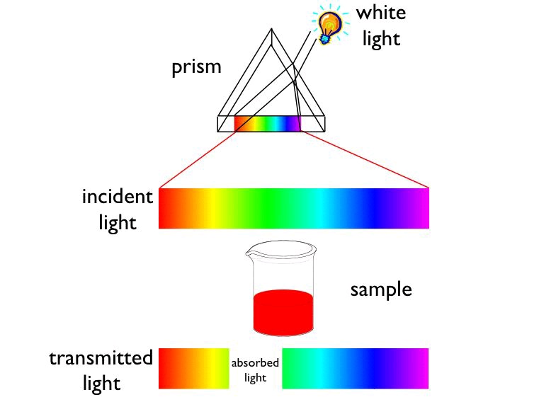

If an object absorbs all
wavelengths of visible light, none reaches our eyes, and it appears black. If it absorbs no visible light, it will look white or colorless. If it absorbs all but orange, the material will appear orange.
We also perceive an orange color when visible light of all colors except blue strikes our eyes.
Orange and blue are complementary colors; the removal of blue from white light makes the light
look orange, and vice versa. Thus, an object has a particular color for one of two reasons: It
transmits light of only that color or it absorbs light of the complementary color.
Figure 4.1.
Complementary colors can be determined using an artist's color wheel. The wheel shows the
colors of the visible spectrum, from red to violet. Complementary colors, such as orange and blue, appear as wedges opposite each other on the wheel.
With our eye, we can make qualitative judgments about the color(s) of light a sample absorbs.
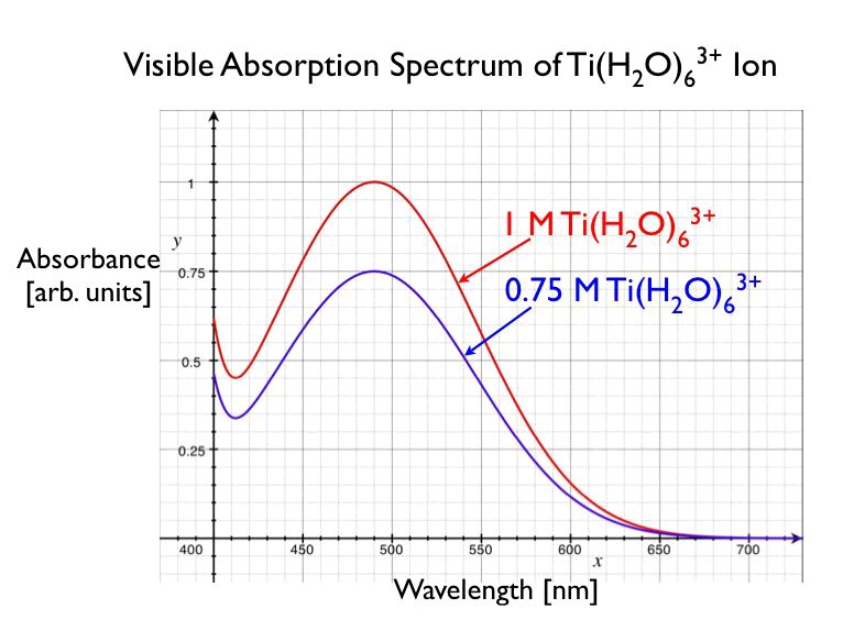
However, given a red solution of [Ti( H 2 O)6]3+ we can not determine if it absorbs green light or if it absorbs all colors of light but red. To quantitatively determine the amount of light absorbed by a sample as a function of wavelength, we will measure its absorption spectrum using a UV-visible
spectrophotometer. Typical absorption spectra of aqueous [Ti( H 2 O)6]3+ solutions are shown below.
Notice the absorption
maximum is at 490 nm. Because the sample absorbs more strongly in the green and yellow
regions of the visible spectrum, it appears red-violet. Measuring the absorption spectrum of a
second, more dilute solution demonstrates that the spectrum changes as a function of the
concentration of the solution. To understand how to use the absorption spectrum as a quantitative tool for chemical analysis, read on!
Spectrophotmetric Basics
The essential components of a spectrophotometer consist of a radiation source, a wavelength
selector (monochromator), a photodetector and read-out device.
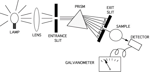
Figure 4.2.
The incident light from a tungsten (visible light source) or deuterium (UV light source) lamp is focused by a lens and passes through an entrance slit. By passing the beam through the
monochromator (either a prism or a diffraction grating) it is separated into monochromatic (i.e., one-color or single-wavelength) light. One particular wavelength of monochromatic light is
selected and allowed to pass through the exit slit into the sample. Light transmitted through the sample is detected by a photodetector which converts the signal to an electrical current which is measured by a galvanometer and sent to a recording device, typically a computer.
The measurement of transmittance (T) is made by determining the ratio of the intensity of
incident ( I 0) and transmitted (I) light passing through pure solvent and sample solutions as a function of wavelength. [Note: The percent transmittance (%T) is obtained by multiplication of T
by 100.] The logarithm of the reciprocal of the transmittance is called the absorbance (A),
A = log (1 / T)
Care must be taken when small values of transmittance are being measured as stray light from
either the room or scattering within the instrument can cause large errors in your readings!
Extracting Quantitative Information
The Beer-Lambert law relates the amount of light being absorbed to the concentration of the
substance absorbing the light and the pathlength through which the light passes:
A = εbc .
In this equation, the measured absorbance (A) is related to the molar absorptivity constant ( ε), the path length (b), and the molar concentration (c) of the absorbing. The concentration is directly proportional to absorbance.
The single largest application of the spectrophotometer is for quantitative analysis. The
prerequisite for such analysis is a known absorption spectrum of the compound under
investigation. Of particular importance is the maximum absorption (at λ max) [Why choose the maximum? Could the choice alter the precision of our experiment? the accuracy?], which can be
easily obtained by plotting absorbance vs. wavelength at a fixed concentration. Next, a series of solutions of known concentration are prepared and their absorbance is measured at λ max. Plotting absorbance vs. concentration, a calibration curve can be determined and fit using linear regression (least-squares fit). An unknown concentration can be deduced by measuring absorbance at the
absorption maximum and comparing it to the standard curve. Caution: The Beer-Lambert Law is
only obeyed (the standard curve is linear) for reasonably dilute solutions. Only those points in the linear range of the standard curve may be used for accurate concentration determination.
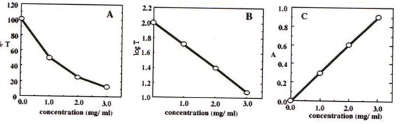
Typical results are shown for the absorbance of [Ti( H 2 O)6]3+ measured at 490 nm.
Table 4.1.
Concentration (mg/mL) %Transmittance Absorbance
0
100.
0
1
50.0
0.301
2
25.0
0.602
3
12.5
0.903
Figure 4.3.
Over the studied range the solutions obey Beer's Law. If a solution has a measured absorbance of 0.450, we can calculate its concentration to be 1.5 mg/mL.
Experimental Procedure
In this experiment, each lab pair will measure the absorbance of CuSO4 at six concentrations. You will create a calibration curve to correlate copper sulfate concentration to absorbance. This curve will be used next week to determine the concentration of an unknown copper sulfate solution and, in turn, the percent yield of a series of chemical reactions.
Materials CuSO4⋅5H2 O distilled water pipette bulb 1cm cuvette 4 - 25 mL volumetric flask for your dilutions
Note: You will be borrowing these and must collect them from your TA. Do not forget to return
the flask at the end of the lab). All students will lose 3 points in that lab section if any go missing!
100 mL volumetric flask for the parent solution (in your drawer)10 mL volumetric pipette or 10
mL graduated cylinder
1. Measure out an appropriate mass of CuSO4⋅5H2 O to get 100ml of ~0.1M solution and record the mass on your report form. Show your calculation to the TA before making the solution.
This is your parent solution. Calculate the molarity using the actual mass measured and record
it.
2. Do the following dilutions and calculate the concentrations for each.
Table 4.2.
Dilution (ml parent : ml total)
0:25 (DI H 2 O)
5:25
10:25
15:25
20:25
25:25 (parent solution)
1. Measure the absorbance of the 6 solutions you have prepared and the unknown given to you by your TA.
Analysis
Plot the concentration as a function of absorbance for your six solutions. Perform a linear
regression analysis and determine the equation of a best-fit line.
PreLab: Spectrophotometry and Data Analysis – Beer’s Law
Hopefully here for the Pre-Lab Name(Print then sign): ___________________________________________________
Lab Day: ___________________Section: ________TA__________________________
This assignment must be completed individually and turned in to your TA at the beginning of lab.
You will not be allowed to begin the lab until you have completed this assignment.
In many of the experiments that you will do throughout the duration of this course you will be
asked to analyze your data by making plots and calculating the best fit line through your data. One program commonly used to analyze data in this fashion is Microsoft Excel ®. The following
exercise will help you through the process used to obtain a plot and linear regression for a set of data.
Suppose you go for a 5 mile run and you tabulate the after each mile as in the following table.
Table 4.3.
Distance Traveled (miles) Time (sec)
1
510
2
1026
3
1548
4
2077
5
2612
Questions:
1. Plot the distance traveled in miles vs. the time in seconds.
2. Use linear regression to obtain a trendline and give the equation obtained in terms of the
variables distance traveled and time and the R-squared value. Comment on the meaning of the
R-squared value and its significance when doing data analysis.
3. Using the equation you obtained by doing linear regression, estimate how long the 6th mile
will take you to run.
4. Assuming this linear trend persists, how far have you run if you finish in 2900 sec.
EXCEL INSTRUCTIONS:
In order to plot this data in excel, you should enter the data exactly as above in to column A
(rows 1-6) and column B (rows 1-6).
To plot the data you will need to go to Insert on the tool bar and then click Chart. A Chart
Wizard will appear. Select XY(Scatter) as the Chart type and choose the sub-type that does not
have any lines connecting the points, then click next.
On Step 2, click on the series tab near the top of the screen and click Add.
You do not need to name the series unless you have multiple plots on one graph, but you can
type in a name if you wish.
To insert the X data, click on the icon at the far left of the x series box.
Select the x values by clicking on the first one and while the left mouse button is down
dragging the mouse down to the last value.
When the values have been selected click the icon again and repeat for the y values. You may
also manually enter the values by separating them with a comma. Don’t forget you need to
remember what units you are using when answering questions.
Click next when you have x and y values entered correctly.
The next step is just entering title information and changing the appearance of your plot; click next when finished.
Choose your chart location and then finish. You now need to place a linear regression line on
your plot.
Right click on a data point and pick add trendline.
Choose linear as the type and click the options tab.
Check the boxes to get the equation and R-squared value and click ok.
Solutions
Chapter 5. Hydrogen and Fuel Cells
Hydrogen and Fuel Cells Experiment
Objective
Build a fuel cell in order to appreciate practically a range of important chemical and physical principles, such as galvanic cells, energy conversion, energy quality, combustion reactions,
water electrolysis and bio-fuels.
Crituique the design in order to improve the efficiency of the fuel cell and to accomplish it
practically
Grading
Pre-lab (10%)
Lab Report (80%)
TA points (10%)
Before Coming to Lab…
Read the lab instructions
Introduction
As the world’s reserves of fossil fuels are diminishing and our awareness of environmental
protection is increasing, we strive to develop alternative ways of energy production. Thus in many countries research into construction of stable and efficient fuel cells has been given high priority.
Indeed, President Bush in his January 28th 2003 State of the Union address, proposed a $1.2
billion fuel-cell research and development program.
Fuel cells are used for direction conversion of the energy of combustion reactions to electrical energy. A possible fuel is hydrogen, which can be produced from water in electrolysis plants
driven by solar cells or windmills. A future interesting fuel source for operation fuel cells might be “bio-fuels” i.e fuels produced from non-fossil organic material such as methane from biogas
plants, alcohol produced by fermentation of sugar or hydrolyzed starch (or, in the not so distant future, perhaps also from enzymatically hydrolyzed cellulose).
Conventional power plants turn approximately 40% of the fuel energy into electricity; we say that the efficiency of the plant is 40%. (Although, in some modern plants surplus heat is reused for district heating thus increasing the actually efficiency somewhat). However, with fuel cells the efficiency of chemical-to-electric energy conversion is unsurpassed, namely about 70% (or even
high in some experimental plants).
U.S. energy dependence is higher today than it was during the “oil shock” of the 1970’s, and oil imports are project to increase. Passenger vehicles alone consume 6 million barrels of oil every day, equivalent 85% of oil imports.
If just 20% of cars used fuel cells, we could cut oil imports by 1.5 million barrels a day.
If every new vehicle sold in the U.S. next year was equipped with a 60kW fuel cell, we would
double the amount of the country’s available electricity supply.
10,000 fuel cell vehicles running on non-petroleum feul would reduce oil consumption by 6.98
million gallons per year.
Fuel cells could dramatically reduce urban air pollution, decrease oil imports, reduce the trade deficit and produce American jobs. The U.S. Department of Energy projects that if a mere 10% of automobiles nationwide were powered by fuel cells, regulated air pollutants would be cut by one million tons per year and 60 million tons of the greenhouse gas carbon dioxide would be
eliminated. DOE projects that the same number of feel cell cars would cut oil imports by 800,000
barrels a day – about 13% of total imports. Since fuel cells run on hydrogen derived from a
renewable source, the fuel cell emissions will be nothing but water vapor.
The Chemistry of a Fuel Cell
A fuel cell is a galvanic cell in which electricity is generated by a combustion reaction. The fuel cell consists of two electrodes between which electrical contact is established by means of an
electrolyte. Oxygen or just plain atmospheric air is fed continuously to the cathode and the fuel is fed continuously to the anode.
The fuel could be any of a vast number of combustible materials, e.g. methane, ethane or ethanol (all organic fuels) hydrogen, hydrazine or sodium borohydride (inorganic fuels). With the
hydrogen burning cell as an example we can describe the chemistry of the cell by the following
reactions:
Anode – at which oxidation of the fuel takes place:
H2 + 2OH- -> 2H2O + 2e-
Cathode – at which reduction of oxygen takes places
½ O2 + H2O + 2e- -> 2OH-
The next reaction for the cell:
H2 + ½ O2 -> H2O
With ethanol as the fuel the matter becomes somewhat more complicated, since ethanol is
oxidized in steps to ethanal, ethanoic acid and carbon dioxide respectively. In an ideally working fuel cell we assume that ethanal and ethanoic acid are further oxidized so that the only carbon compound of the overall process is carbon dioxide. We have not succeed ( by simple chemical
tests) to detect either ethanol or ethanoic acid (or rather ethanoate due to the strongly basic electrolyte solution) as intermediate products in our own cells. However we still suggest a three-step oxidation of ethanol(and at the same time admitting that the last step is dubious):
Anode:
Step 1: CH3CH2OH + 2 OH- -> CH3CHO + 2 H2O + 2e-
Step 2: CH3HO + 2 OH- -> CH3COOH + H2O + 2 e-
Step 3: CH3COOH +8 OH- -> 2 CO2 + 6 H2O + 8 e-
Sum: CH3CH2OH + 12OH- -> 2 CO2 + 9 H2O + 12 e-