ELEC 301 Projects Fall 2005 by Danny Blanco, et al - HTML preview
Download the book in PDF, ePub, Kindle for a complete version.
it could improve the statistical accuracy of the GMM when decomposing polyphonic test signals.
Increasing the scope
In addition to training the GMM for other players on the three instruments used in this project, to
truly decode an arbitrary musical signal, additional instruments must be added. This includes
other woodwinds and brass, from flutes and double reeds to french horns and tubas, to strings and
percussion. The GMM would likely need to extensively train on similar instruments to properly
distinguish between them, and it is unlikely that it would ever be able to distinguish between the
sounds of extremely similar instruments, such as a trumpet and a cornet, or a baritone and a
euphonium. Such instruments are so similar that few humans can even discern the subtle
differences between them, and the sounds produced by these instruments vary more from player to
player than between, say, a trumpet and a cornet.
Further, the project would need to include other families of instruments not yet taken into
consideration, such as strings and percussion. Strings and tuned percussion, such as xylophones,
produce very different tones than wind instruments, and would likely be easy to decompose.
Untuned percussion, however, such as cymbals or a cowbell, would be very difficult to add to this
project without modifying it, adding features specifically to detect such instruments. Detecting
these instruments would require adding temporal features to the GMM, and would likely entail
adding an entire beat detection system to the project.
Improving Pitch Detection
For the most part, and especially in the classical genre, music is written to sound pleasing to the
ear. Multiple notes playing at the same time will usually be harmonic ratios of one another, either
thirds, or fifths, or octaves. With this knowledge, once we have determined the pitch of the first
note, we can determine what pitch the next note is likely to be. Our current system detects the
pitch at each window without any dependence on the previously detected note. A better model
would track the notes and continue detecting the same pitch until the note ends. Furthermore,
Hidden Markov Models have been shown useful in tracking melodies, and such a tracking system
could also be incorporated for better pitch detection.
8.13. Acknowledgements and Inquiries*
The team would like to thank the following people and organizations.
Department of Electrical and Computer Engineering, Rice University
Richard Baraniuk, Elec 301 Instructor
William Chan, Elec 301 Teaching Assistant
Music Classification by Genre. Elec 301 Project, Fall 2003. Mitali Banerjee, Melodie Chu,
Chris Hunter, Jordan Mayo
Instrument and Note Identification. Elec 301 Project, Fall 2004. Michael Lawrence, Nathan
Shaw, Charles Tripp.
Auditory Toolbox. Malcolm Slaney
Netlab. Neural Computing Research Group. Aston University For the Elec 301 project, we gave a poster presentation on December 14, 2005. We prefer not to provide our source code online, but if you would like to know more about our algorithm, we
welcome any questions and concerns. Finally, we ask that you reference us if you decide to use
any of our material.
8.14. Patrick Kruse*
Patrick Alan Kruse
Figure 8.8.
Patrick Kruse
Patrick is a junior Electrical Engineering major from Will Rice College at Rice University.
Originally from Houston, Texas, Patrick intends on specializing in Computer Engineering and
pursuing a career in industry after graduation, as acadamia frightens him.
8.15. Kyle Ringgenberg*
Kyle Martin Ringgenberg
Figure 8.9.
Kyle Ringgenberg
Originally from Sioux City, Iowa... Kyle is currently a junior electrical engineering major at Rice
University. Educational interests rest primarily within the realm of computer engineering. Future
plans include either venturing into the work world doing integrated circuit design or remaining in
academia to pursue a teaching career.
Outside of academics, Kyle's primary interests are founded in the musical realm. He's performs
regularly on both tenor saxophone and violin under the genres of jazz, classical, and modern. He
also has a strong interest in 3d computer modeling and animation,which has remained a self-
taught hobby of his for years. Communication can be established via his personal website,
www.KRingg.com, or by the email address listed under this Connections course.
8.16. Yi-Chieh Jessica Wu*
Figure 8.10.
Jessica Wu
Jessica is currently a junior electrical engineering major from Sid Richardson College at Rice
University. She is specializing in systems and is interested in signal processing applications in
music, speech, and bioengineering. She will probably pursue a graduate degree after Rice.
Solutions
Chapter 9. Accent Classification using Neural Networks
9.1. Introduction to Accent Classification with Neural
Networks*
Overview
Although seemingly subtle, accents have important influences in many areas – from business, to
sociology, technology, security, and intelligence. While much linguistic analysis has been done on
the subject matter, very little work has done with regards to potential applications.
Goals
The goal of this project is to generate a process for accurate accent detection. The algorithm
developed should have the flexibility to choose how many accents to differentiate between.
Currently, the algorithm is aimed at differentiating accents by languages, rather than regions, but
should be able to conform to the latter as well. Finally, the application should produce an output
showing the relative strength of a speaker's primary accent compared to the rest in the system.
Design Choices
The agreed-upon option for achieving the desired flexibility in the project's algorithm is to use a
neural network. A neural network is a matrix containing weights that correspond to how certain
parameters fed to the network tie the inputs to the outputs. Parameters of known inputs with
corresponding outputs are fed to the network to train it. Training the network produces the
weighted matrix, to which test samples can then be fed. This provides a powerful and flexible tool
that can be used to generate the desired algorithm.
Utilizing this limits the project group only by the amount of overall samples collected to train the
matrix with, and how they are defined. For this project, approximately 800 samples from over 70
people have been collected for the purposes of training and testing. The group of language-based
accents to test with consists of American Northern English, American Texan English, Farsi,
Russian, Mandarin, and Korean.
Applications
Potential applications for this project are incredibly diverse. One example might be for tagging
information about a subject for intelligence purposes. The program could also be used as a
potential aid/error check for voice-recognition based systems such as customer service or
bioinformatics in security systems. The project can even aid in showing a student's progress in
learning a foreign language.
9.2. Formants and Phonetics*
Taking the FFT (Fast Fourier Transform) of each voice sample outputs its frequency spectrum. A
formant is one of four highest peaks in a spectrum sample. From the frequency spectrums, the
main formants can be extracted. It is the location of these formants along the frequency axis that
define a vowel sound. There are four main peaks between 300 and 4400 Hz, this bandwidth is
where the strongest formants for human speech occur. For the purposes of this project, the group
is to extract the frequency values of only the first two peaks since they provide the most
information in terms of what the vowel sound is. Since all vowels follow constant and
recognizable patterns in these two formants, the changes along an accent can be recorded with a
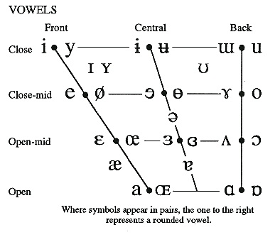
high degree of accuracy. Figure 1 shows this pattern between the vowel sounds and formant
frequencies.
Figure 9.1. The IPA Vowel Chart
The first formant (F1) is dependant on whether a vowel sound is more open or closed, so on the
chart, F1 varies along the y axis. F1 increases in frequency as the vowel becomes more open and


decreases to its minimum as the vowel sound closes. The second formant (F2), however, follows
along the x-axis. Thus, it varies depending on whether a sound is made in the front or the back of
the vocal cavity. F2 increases in frequency the farther forward that a vowel is and decreases to its
minimum as a vowel moves to the back. Therefore, each vowel sound has unique, characteristic
formant values for its first two formants. With this in mind, it means that theoretically, across
many speakers, the same frequency values for the first two formant locations should hold as long
as they are making the same vowel sound.
Sample Spectograms
Figure 9.2. a as in call
The first and second formant have similar values
Figure 9.3. i as in please
Very high f2 and small f1
9.3. Collection of Samples*
Choosing the sample set
We decided that one sample for each of the English vowels on the IPA chart would be a fairly
thorough representative sample of each individual’s accent. With the inclusion of the two
diphthongs that we also extracted, we took 14 vowel samples per person. We used the following
paragraph in each recording; there are at least 4 instances of each vowel sound located throughout
it.
Figure 9.4.
Phonetic Background
(Please i, call a, Ste-ε, -lla ə, Ask æ, spoons u , five ai, brother ə^, Bob α, Big I, toy oi, frog ν, go o, station e)

The vowels in bold are the ones we decided to extract; we determined that these would provide the
cleanest formants for the whole paragraph. For example, the ‘oo’ in ‘spoons’ was chosen due to
the ‘p’ that precedes the vowel. The ‘p’ sound creates a stop of air, almost like a vocal ‘clear’. A
‘t’ will also do this, which explains our choice of the ‘a’ in ‘station’.
Figure 9.5. Spoons
The stop made by the 'p' is visible as a lack of formants
The two diphthongs present are the ‘ai’ from ‘five’ and ‘oi’ from ‘toy’. In these samples, the
formant values move smoothly from the first vowel representation to the second.
The vowel samples that we cut out of the main paragraph ended up being about 0.04 seconds each
with diphthongs being much longer to capture the entire sample transition.
9.4. Extracting Formants from Vowel Samples*
For each vowel sample we needed to extract the first and second formant frequencies. To do this
we made a function in MATLAB that we could then apply to each speaker's vowel samples
quickly. In an ideal world with clear speech this would be a straightforward process, since there
would be two or more peaks on the frequency spectrum with little oscillation. The formants would
be simply be the locations of the first two peaks.
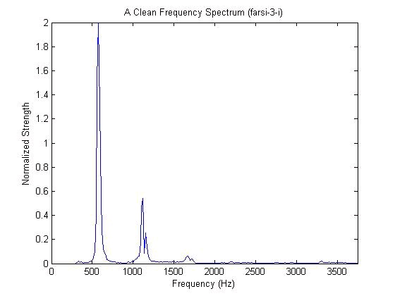
Figure 9.6.
However, very few of the samples are this clear. If the formants do not stay constant during the
entire clip, then the formant peaks have smaller peaks on them. In order to solve this problem we
did three things. First we cut the samples into thirds, found the formants in each division, and then
averaged the three values for a final formant value. Second, we ignored frequencies below 300 Hz
which correspond to frequencies made when the human vocal tract makes a sound. Finally we
filtered our frequency spectrum data to remove noise from the peaks. We also experimented with
cubing the spectrum, but the second formant was generally small and cubing the signal made it
harder to find. As a guide for the accuracy of our answer we used the open source application
Praat. Praat can accurately find the formants using a more advanced techniques.
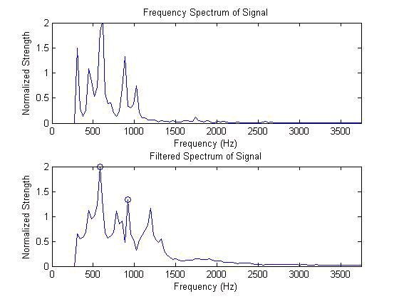
Figure 9.7.
With the aid of Praat, the first and second formants should be 569.7 Hz and 930.3 Hz. In the
unfiltered spectrum there is a strong peak just above 300Hz which does not correspond to a
formant, in the filtered spectrum it is removed.
To locate the first formant we started by finding the maximum value in the spectrum. However,
sometimes the second formant is stronger than the first, so we looked for another peak before this
first guess above a threshold (1.5 on the normalized scale). If a peak could not be found before the
maximum to be the first formant, then we had to search for a second formant beyond the first. We
did this in the exact same manner as finding the first, but we only looked at the part of the
spectrum above the minimum immediately following the first peak. We found this minimum with
the aid of the derivative.
This function was used on each vowel sample to generate an accent profile for each speaker. The
profile consisted of the first and second formants of the speaker's 14 vowels in a column vector.
9.5. Neural Network Design*
To implement our neural network we used the Neural Network Toolbox in MATLAB. The neural
network is built up of layers of neurons. Each neuron can either accept a vector or scalar input (p)
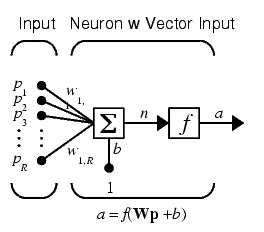

and gives a scalar output (a). The inputs are weighted by W and given a bias b. This results in the
inputs becoming Wp + b. The neuron transfer function operates on this value to generate the final
scalar output a.
Figure 9.8. A MATLAB Neuron that Accepts a Vector Input
Our network used three layers of neurons, one of which is required by the toolbox. The final layer,
output layer, is required to have neurons equal to the size of the output. We tested five accents, so
our final layer has 5 neurons. We also added two "hidden" layers, which operate on the inputs
before they are prepared as outputs, each of which have 20 neurons.
In addition to configuring the network parameters, we had to build the network training set. In our
training set we had 42 speakers: 8 Northern, 9 Texan, 9 Russian, 9 Farsi, and 7 Mandarin. An
accent profile was created for each of these speakers as discussed and compacted into a matrix.
Each profile was a column vector, so the size was 42 x 28. For each speaker we also generated an
answer vector. For example, the desired answer for a Texan accent is [0 1 0 0 0]. These answer
vectors were also combined into an answer matrix. The training matrix and the desired answer
matrix were given to the neural network which trained using traingda (gradient descent with
adaptive learning rate backpropogation). We set the goal for the training function to be a mean
square error of .005.
We originally configured our neural network to use neurons with a linear transfer function
(purelin), however when using more than three accents at a time we could not reduce the mean
square error to .005 The error approached a limit, which increased as the number of accents we
included increased.
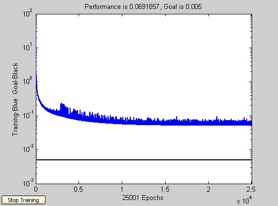
Figure 9.9. Linear Neuron Transfer Function
Figure 9.10. Linear Neurons Training Curve
So, at this point we redesigned our network to use non-linear neurons (tansig).
Figure 9.11. Tansig Neuron Transfer Function
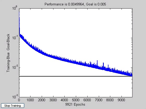
Figure 9.12. Tansig Neurons Training Curve
After the network was trained we refined our set of training samples by looking at the network's
output when given the training matrix again. We removed a handful of speakers to arrive at our
present number of 42 because they included an accent we weren't explicitly testing for. These
consisted of speakers who sounded as if they did not learn American English, but British English.
These final two figures show an image representation of the answer matrix and the answers given
by the trained matrix. In the images, grey is 0 and white is one. Colors darker than grey represent
negative numbers.
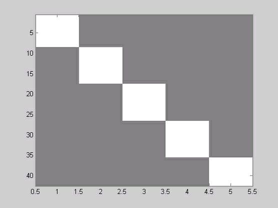
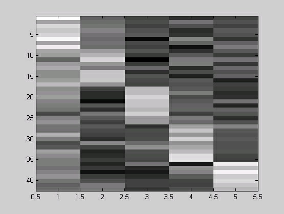
Figure 9.13. Answer Matrix
Figure 9.14. Trained Answers
9.6. Neural Network-based Accent Classification
Results*
Results
The following are some example outputs from the neural network from various test speakers. The
output displays relative strengths of different types of accents prevalent in a particular subject. All
test inputs were not used in the training matrix. Overall, approximately 20 tests were conducted
with about an 80% success rate. Those that failed tended to with good reason (either inadequate
recording quality, or speakers who did not provide accurate information about what their accent is
comprised of – a common issue with subjects who have lived in multiple places).
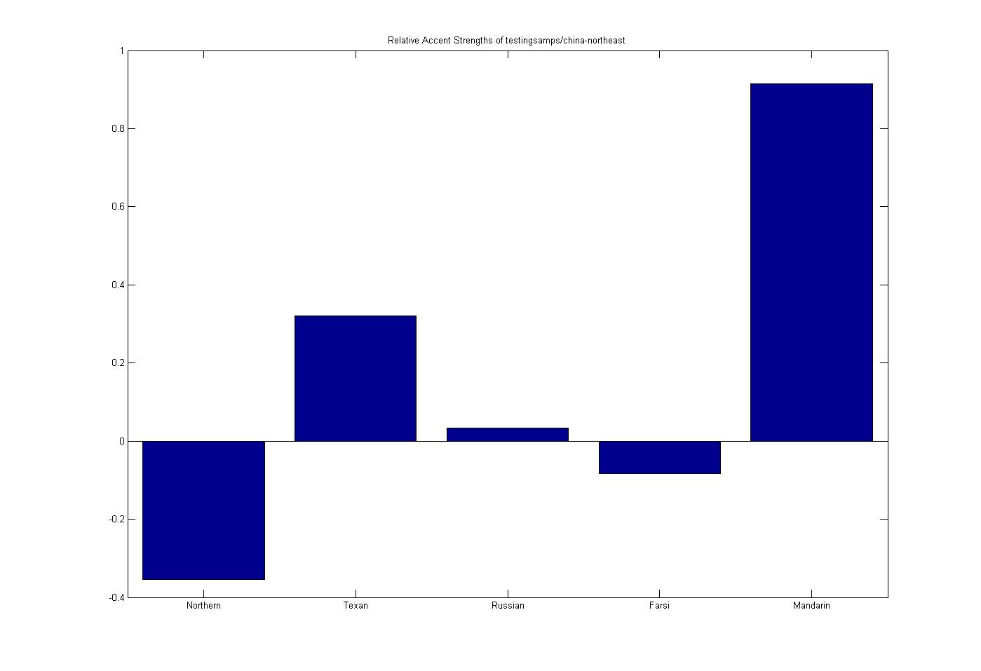
The charts below show accents in the following order: Northern US, Texan US, Russian, Farsi, and
Mandarin
Test 1: Chinese Subject
Figure 9.15. Chinese Subject
Chinese Subject (accent order: Northern US, Texan US, Russian, Farsi, and Mandarin)
(This media type is not supported in this reader. Click to open media in browser.)
Here our network has successfully picked out the accent of our subject. Secondarily, the network
picked up on a slight Texan accent, possibly showing the influence of location on the subject (The
sample was recorded in Texas).
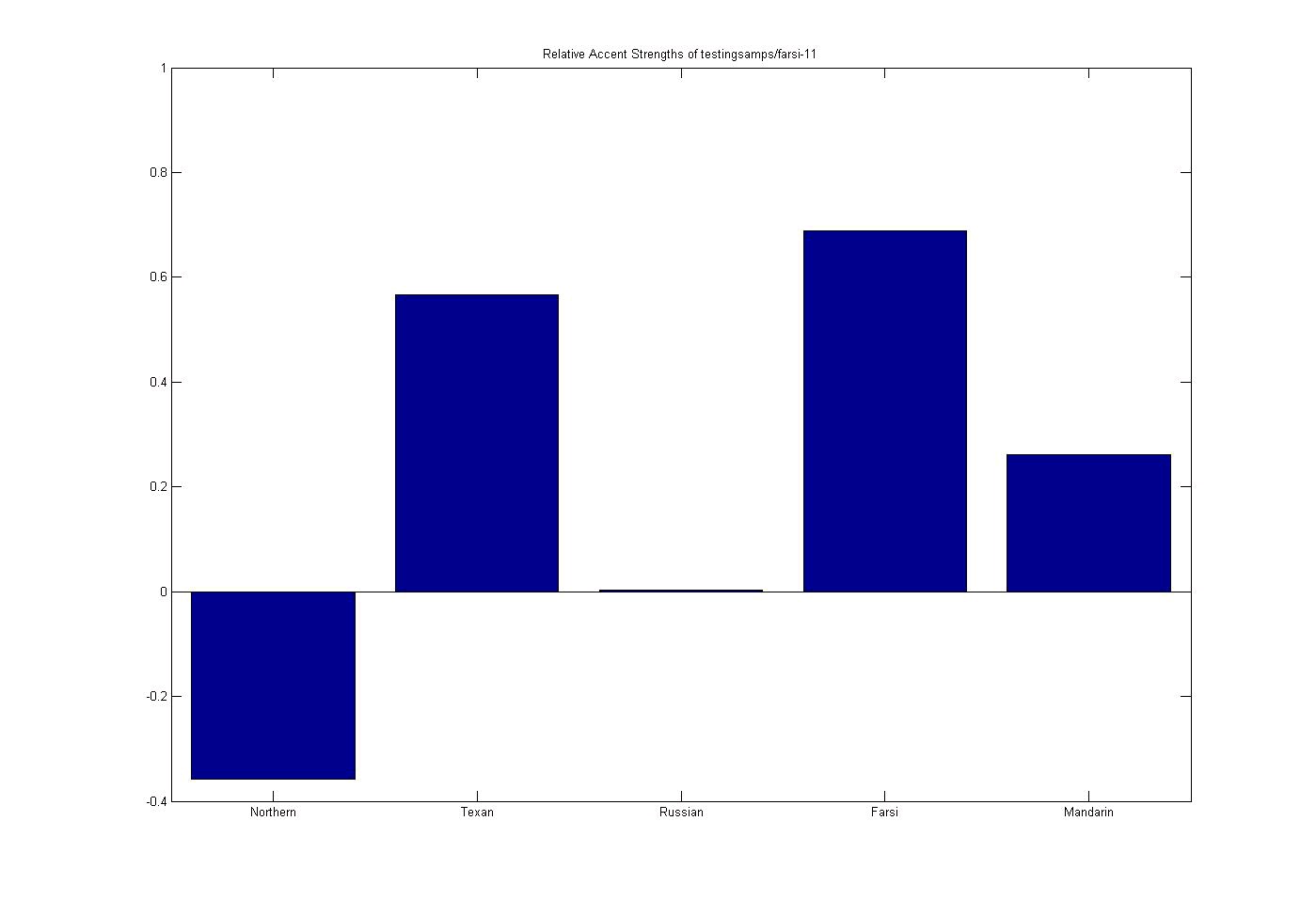
Test 2: Iranian Subject
Figure 9.16. Iranian Subject
Iranian Subject (accent order: Northern US, Texan US, Russian, Farsi, and Mandarin)
(This media type is not supported in this reader. Click to open media in browser.)
Again our network has successfully picked out the accent of our subject. Once again, this sample
was recorded in Texas, which could account for the secondary influence of a Texan accent in the
subject.
Test 3: Chinese Subject
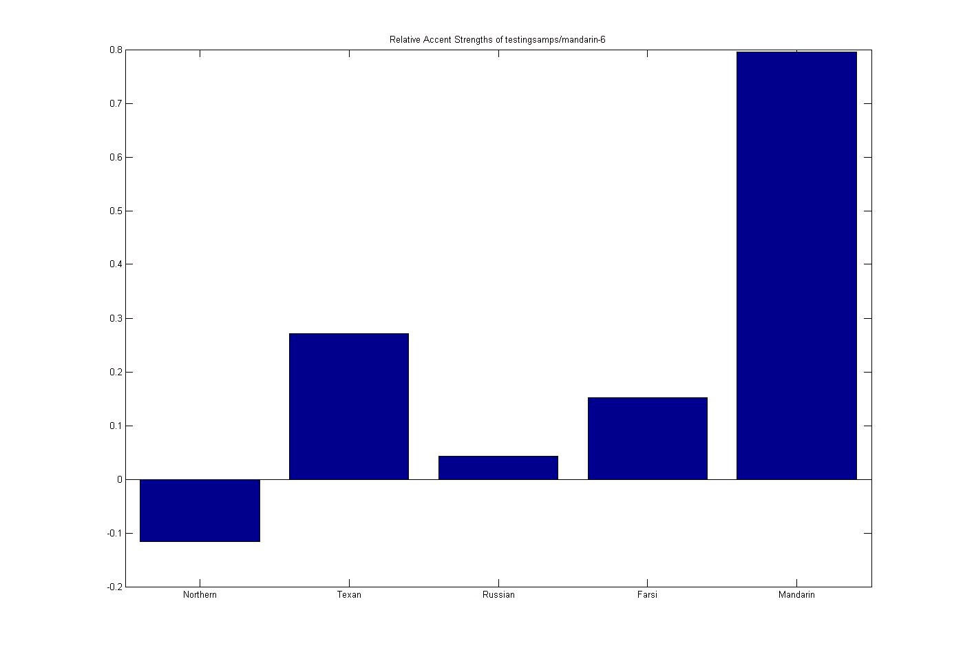
Figure 9.17. Chinese Subject
Chinese Subject (accent order: Northern US, Texan US, Russian, Farsi, and Mandarin)
(This media type is not supported in this reader. Click to open media in browser.)
Once again, the network successfully picks up on the subjects primary accent as well as influence
of a Texan accent (this sample was also recorded in Texas).
Test 4: Chinese Subject
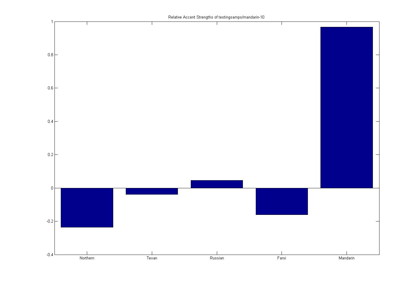
Figure 9.18. Chinese Subject
Chinese Subject (accent order: Northern US, Texan US, Russian, Farsi, and Mandarin)
(This media type is not supported in this reader. Click to open media in browser.)
A successful test showing little or no influence from other accents in the network.
Test 5: American Subject (Hybrid of Regions)
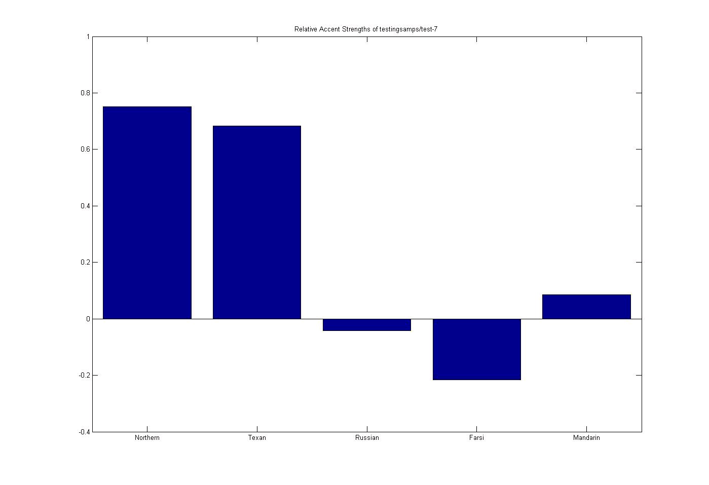
Figure 9.19. American Subject (Hybrid)
American Subject - Hybrid (accent order: Northern US, Texan US, Russian, Farsi, and Mandarin)
(This media type is not supported in this reader. Click to open media in browser.)
Results from a subject who has lived all over -- mainly in Texas, who's accent appears to sound
more Northern (which seems relatively true if one listens to the source recording).
Test 6: Russian Subject
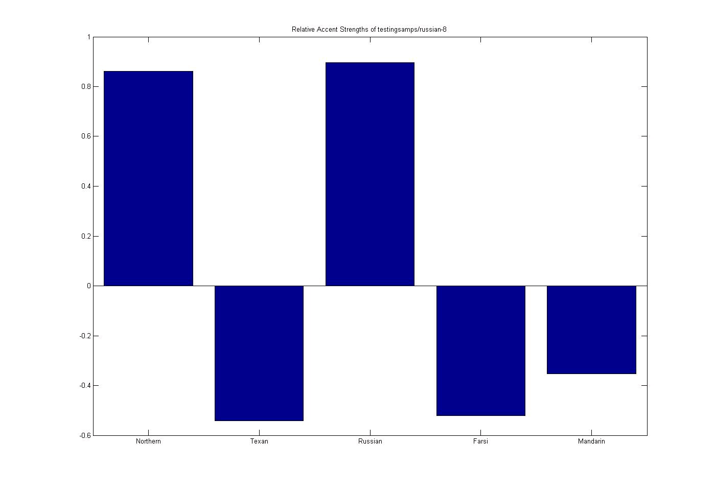
Figure 9.20. Russian Subject
Russian Subject (accent order: Northern US, Texan US, Russian, Farsi, and Mandarin)
(This media type is not supported in this reader. Click to open media in browser.)
Successful test of a Russian subject with strong influences of a Northern US accent.
Test 7: Russian Subject
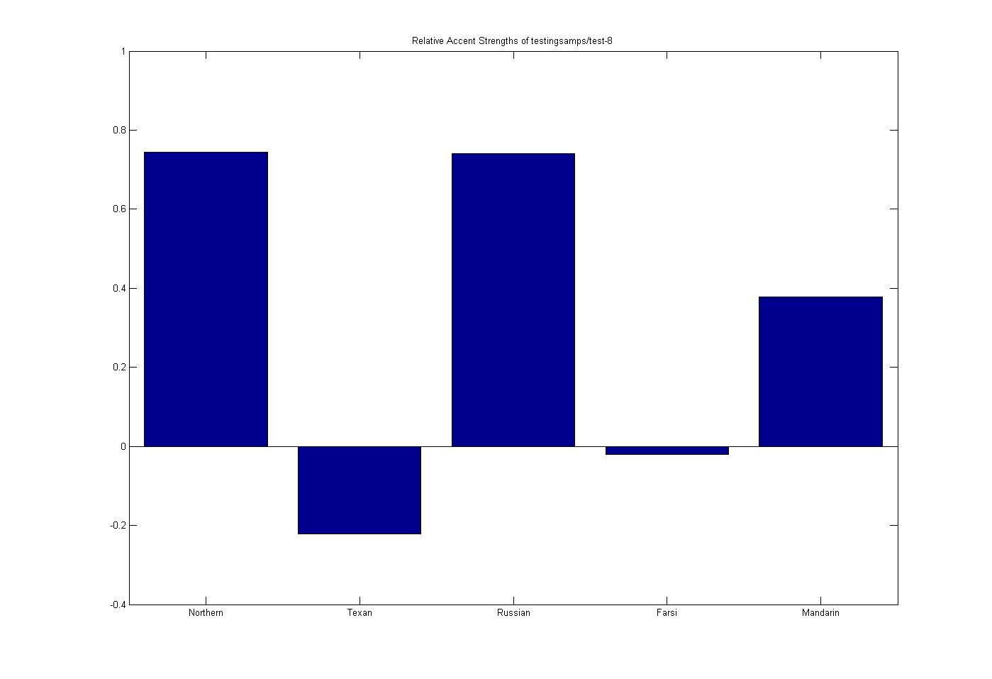
Figure 9.21. Russian Subject
Russian Subject (accent order: Northern US, Texan US, Russian, Farsi, and Mandarin)
(This media type is not supported in this reader. Click to open media in browser.)
Another successful test of a Russian subject with strong influences of a Northern US accent.
Test 8: Cantonese Subject
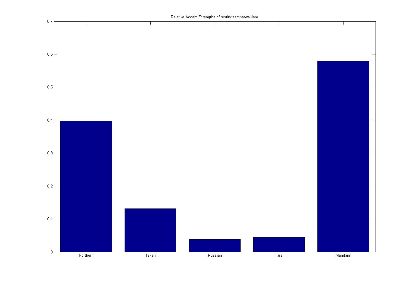
Figure 9.22. Cantonese Subject
Cantonese Subject (accent order: Northern US, Texan US, Russian, Farsi, and Mandarin)
(This media type is not supported in this reader. Click to open media in browser.)
Successful region-based test of a Cantonese subject who has been living in the US.
Test 1: Korean Subject
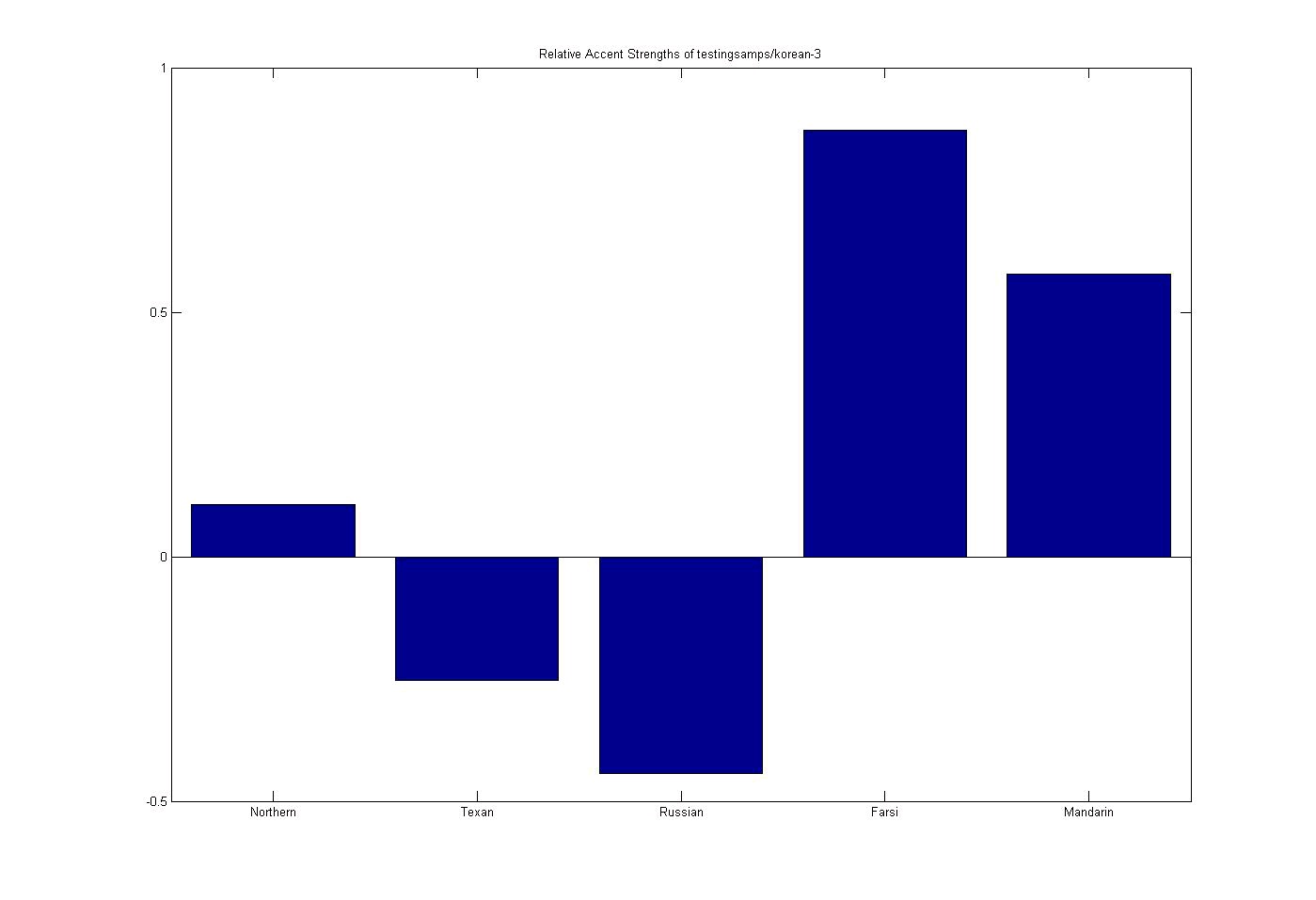
Figure 9.23. Korean Subject
Korean Subject (accent order: Northern US, Texan US, Russian, Farsi, and Mandarin)
(This media type is not supported in this reader. Click to open media in browser.)
An interesting example of throwing an accent at the network that doesn't fit into any of the
categories.
9.7. Conclusions and References*
Conclusions
Our results showed that vowel formant analysis provides accurate information on a person’s
overall speech and accent. However, the differences are not in how speakers make the vowel
sounds, but by what vowel sounds are made when speaking certain letter groupings. They also
showed that neural networks are a viable solution for generating an accent detection and
classification algorithm. Because of the nature of neural networks, we can improve the
performance of the system by feeding more training data into the network. We can also improve
the performance of our system by using a better formant detector. One suggestion we received
from the creator of Praat was to use pre-emphasis to make the formant peaks more obvious, even
if one formant peak is on another formant's slope.
Acknowledgements
We would like to thank all the people who allowed us to record their voices and Dr. Bill for<