ELEC 301 Projects Fall 2005 by Danny Blanco, et al - HTML preview
Download the book in PDF, ePub, Kindle for a complete version.
reduced the number of samples and the number of angles. Our shrinkPR code takes the original PR
matrix, a matrix whose columns are the projections, and outputs a smaller PR matrix with fewer
samples and angles. It also creates a column vector, theta, which contains the angles of the
corresponding projections.
Filtersinc
This code takes in the PR matrix and outputs the filtered PR matrix.
Figure 5.18.
It creates the ramp filter |ω| and multiplies it with the FFT of each projection. It then takes the
IFFT of each filtered projection.
Backproject
Backproject implements the discrete approximation of :
Figure 5.19.
This code backprojects each of the filtered projections over the image plane and sums them
together to produce the final reconstructed image. In order to implement the continuous function
given discrete data points, the “round” function was used, effectively interpolating the data.
Representative Results
The following are reconstructed images:
1500 samples per projection and 360 angles:

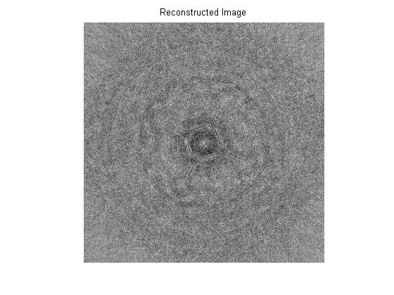
Figure 5.20.
From this image you can easily see the original object.
1100 samples per projection and 360 angles:
Figure 5.21.
This image is not as clear since fewer samples were used.
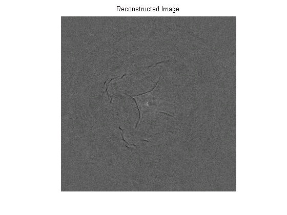
1500 samples and angles 1-180.
Figure 5.22.
From this image you can see the left half of the object since we used the first half of the
projections.
5.7. Conclusions and References*
Conclusions
Using the terahertz reflected waveforms, we were able to measure the projections and reconstruct
the original image. This process was completed in two steps. In the first, inverse and Wiener
filtering were used to deconvolve the data from the reference pulse to obtain the actual projections
of the test object. In the second, the Filtered Backprojection Algorithm featuring the Fourier Slice
Theorem was used to filter the projections using a ramp filter and backproject the result over the
image plane, thus reconstructing the image of the object.
As far as the deconvolution part of the project concerns, the regularized inverse filter gives better
results than Wiener filtering, as already pointed out. Care should be exercised when picking the
regularized parameter γ, so as not to increase the noise level of the resulting signal. Usually, this
is a case-dependent procedure that takes numerical experimentation. It should be noted that the
original data at hand were of very good quality with low noise level. Thus the results of Wiener
filtering were worse than those obtained by inverse filtering.
For the reconstruction part, it was found that the number of projection angles used was vital to the
clarity of the final image. We were able to greatly downsample the data and still maintain image
quality to a certain point. Due to the size of the data, the algorithms ran for minutes.
Future Work
Much potential for future improvement and implementation is possible using this method of
computerized tomography. Advanced deconvolution methods featuring wavelets for efficient
noise reduction can be used for isolating the projections out of the measured waveforms.
Furthermore, it seems reasonable to cut-off the first part of each measured waveform since it only
contains noise and no useful information for the image reconstruction. This can be accomplished
by appropriately windowing the raw measurements before any other manipulations takes place.
Due to the linear nature of the process, different algorithm code could have been written to start
reconstructing the image immediately after the first projection had been calculated. This and other
efficiency tools could be implemented to greatly increase the speed of the overall reconstruction,
making the process applicable for real-time use.
References
J. Pearce, H. Choi, D. M. Mittleman, J. White, and D. Zimdars, Opt. Lett. 30, 1653 (2005).
A. C. Kak and M. Slaney, Principles of Computerized Tomographic Imaging (IEEE Press, 1988).
J. S. Lim, Two- Dimensional Signal and Image Processing (Prentice- Hall Inc., 1990).
D. M. Mittleman, S. Hunsche, L. Bovin, and M. C. Nuss, Opt. Lett. 22, 904 (1997).
B. B. Hu and M. C. Nuss, Opt. Lett., 20, 1716 (1995).
5.8. Team Incredible*
Agathoklis Giaralis is a Civil and Environmenal Engineering PhD candidate.
Paul Campbell is an electrical engineering, economics and pre-med junior at Martel College.
Warren Scott is an electrical engineering and economics junior at Martel College. He is the son of the famous statistics professor Dr. Scott.
Debbie Miller is a CAAM senior from Will Rice College.
Solutions
Chapter 6. Filtering and Analysis of Heart Rhythms
6.1. Introduction to Electrocardiogram Signals*
Abstract
Every year the leading cause of death among Americans is Coronary heart disease (CHD). CHD
typically accounts for approximately 466,000 deaths each year with half of those deaths occurring
before the patient is able to reach a hospital. According to figures by the American Heart
Association, patients who experience a full cardiac arrest in an area where EMS response times
are long may have only a 1 to 2 percent chance of survival. With effective bystander CPR and
prompt response by EMS survival rates increase to around 30 percent. Through advancements in
DSP and portable electronics Automatic External Defibrillators (AEDs) now allow for a whole
new level of care. Prompt action by trained bystanders has led to survival rates approaching 75
percent in some areas employing Public Access Defibrillators (PADs). Rice University uses AEDs
on campus and with their assistance Rice EMS has managed to maintain a survival rate of 60
percent for patients in full cardiac arrest while for the greater Houston area it is closer to 12
percent.
6.2. Medical Background*
The heart rhythm as detected by an ECG is the result of the conduction system which is used by
the heart to coordinate the heart beat. The electrical impulse is started by the SA node at the top of
the heart. At this point the conduction system of the heart passes the impulse across both atria (top
chambers of the heart) and to the AV node. The AV node acts as a time delay and then passes the
impulse on to the conduction system in the Ventricles (lower chambers of the heart). The
ventricles are larger than the atria because they actually pump the blood out of the heart and to the
lungs or the rest of the body. Due to their larger size their depolarization produces the largest
deflection on the ECG reading. This large deflection is referred to as the ventricular complex or
the QRS complex. After the heart is done contracting the tissue must repolarize so that it will be
ready to contract again. This repolarization shows up on the monitor as the "T" wave, or the final wave after the large QRS complex.
The two lethal rhythms mentioned earlier, V-Tach and V-Fib, both cause death by interfering with
the standard electrical coordination of the heart.
V-Tach is a rhythm characterized by a very rapid succession of ventricular complexes. In this
rhythm the heart beats at a rate between 100 and 250 beats per minute. On the monitor you will
see the QRS complex, but due to the fast rate of the rhythm there is no flat period for effective
repolarization. This rhythm is so fast in fact that the Ventricles will begin to contract before
they have had time to actually fill with blood. This is called Pulseless Ventricular Tachycardia.
Once a patient has gone into Pulseless Ventricular Tachycardia, they have only a manner of
minutes before the drop to asystole and their chances of survival plummet.
V-Fib occurs when the electrical system of the heart becomes exceedingly discoordinated. It is
characterized only by random electrical activity without the presence of a pulse. If this rhythm
is present immediate defibrillation is needed.
If either of these rhythms is left untreated they will rapidly degenerate to asystole or flatline. In
asystole the electrical activity of the heart has stopped and defibrillation is no longer capable of
restarting it. At this point the only hope for survival is aggressive pharmaceutical action through
Advanced Cardiac Life Support algorithms, but even these methods are often ineffective.
In addition to identifying cardiac rhythms that present the possibility of death within the next few
minutes, signal analysis could also identify potentially life threatening conditions before they
reach a state of cardiac arrest. Acute Myocardial Infarctions (AMIs) or Heart Attacks are among
the top causes of death in the United States. While many people become aware of their AMI
through clinical signs such as chest pain, other conditions such as Diabetes or pain from other
illnesses may mask the presence of an AMI. In the hospital an AMI can be detected through its
effect on the conduction system of the heart as shown by an ECG. An active AMI will result in a
lack of Oxygen to some of the myocardium. The ischemic tissue has different conductive
properties; as a result of these changes the T-wave of a patient suffering from Ischemia in the
Myocardium will be inverted. By detecting this rhythm we would allow patients to be alerted of
their problem before they have reached a state of full arrest.
With the increasing use of electrocardiograms and the application of devices such as
defibrillators, proper measurement and identification of ECG signals is extremely important.
However with such signals on the order of microvolts, significant levels of noise corruption make
this very difficult. Having proper filters to remove such noise and allow for proper signal
identification is crucial. This project aims to apply filtering algorithms in hopes of identifying
some of the most common types of ECG signals.
In addition to V-Tach and V-Fib the program identifies the following rhythms:
Sinus is the normal rhythm found, 60 to 100 BPM with a flat period between QRS complexes
for repolarization.
Inverted T-wave is a normal sinus rhythm were the final wave after the QRS complex has
inverted in polarity, this condition is indicative of a lack of Oxygen to the heart as caused by a
heart attack.
Asystole - is a lack of electrical activity shown by a flatline on the ECG readout.
Figure 6.1.
Figure 6.2.
Figure 6.3.
6.3. Block Diagram/Method*
The project group began by obtaining MATLAB data on these five types of ECG signals. The
signals obtained might be thought of as the ideal; that is they were completely free of noise,
perfectly smooth, textbook examples of what each type of signal might look like. A random noise
signal was then generated by use of a random number generator. The level of noise could be
varied by adjusting the amplitude of this noise signal. The noise signal was then added to the ideal
signals to create a simulation of the type of measurement that might be found in the real world.
The group then applied filters and identification algorithms to see if the original signal could be
correctly identified.
Our identification method worked as follows. To reduce noise we convolved the unknown signal
with a sinc function of width seven. Seven was chosen because smaller values did not have
adequate noise reduction and larger values had the adverse effect of essentially “smoothing out”
the signal to too great a degree. We then took an inner product of the filtered signal with all of the
idealized signals. Whichever inner product was the greatest we took to correspond with the correct
signal. That is to say that if the inner product of the unknown signal and the sinus rhythm was
greater than the inner product of the unknown signal with any other of our ideal signals we take
the unknown rhythm to be a sinus rhythm. For flatline we simply stated that if the maximum value
of the signal does not exceed some threshold our cardiac rhythm is flatline.
Figure 6.4.
Analysis of pulse rates were done exclusively in the time domain. We low pass filtered the signal
just as we did when we were trying to identify the type of rhythm. We then found the maximum
value for the given cardiac complex and set a threshold at 80% of that. We can then count the
number of times we exceed that value in a minute.
6.4. Sample Outputs*
The original, unaltered Sinus wave at 80 BPM.
Figure 6.5.
White noise added to the 80 BPM Sinus signal.
Figure 6.6.
The output of the noisy signal sent through a low pass filter.
Figure 6.7.
Output of the matched filter for the given input.
Figure 6.8.
6.5. Overall Results and Conclusions*
Using a function to repeatedly analyze ECGs with our algorithm, we obtained rates of correctly
identifying the right type of rhythm and heart rate for specified noise levels. We then plotted these
rates versus the corresponding SNR value for each noise level to see how much noise we could
tolerate before we could no longer accurately detect the signal’s information. Below are these
particular graphs for an 80 BPM Sinus wave, a 100 BPM Inverted T wave, and a 108 BPM
Ventricular Tachycardia wave.
Figure 6.9.
Figure 6.10.
Figure 6.11.
Figure 6.12.
Figure 6.13.
Figure 6.14.
As shown in the graphs, all signals can be correctly identified with a SNR as low as 4, at which
point the Sinus wave starts to look like a Ventricular Tachycardia wave due to noise. The other
two signals we tested correctly identify the rhythm all the way down to a SNR of about 1.5. As far
as heart rate goes, the Sinus and Inverted T wave always calculate the correct hear rate within two
beats per minute for all signals with a SNR as low as 3, while a Ventricular Tachycardia signal can
only do so. For practical purposes the one to two beat deviation in beats per minute may be
considered negligible as all patients exhibit slight variances in heartrate from one moment to the
next and such a small variance is insignificant for medical purposes anyway.
The fact that the filter and the deciphering algorithm can tolerate such low signal to noise ratios
shows great promise. Though this success rate may be lowered slightly as we add more signal
types to be identified, it seems fairly certain that even for a relatively large number of signal types
we would still be able to identify the correct rhythm for any reasonable SNR value.
6.6. MATLAB Analysis Code*
Click here to download a function that takes the noisy signals and runs it through a low pass filter.
Click here to download a function that takes the cleaned signal and runs it through the matched filter.
Click here to download a function that performs the convolution for each branch of the matched filter.
6.7. Group Members*
6.7. Group Members*
Grant Heberton
Lovett College
Sophomore
ELEC Major
heberton@rice.edu
Robert McArthur
Lovett College
Sophomore
ELEC Major
robertm@rice.edu
Anish Patel
Lovett College
Junior
ELEC Major
anishp@rice.edu
Solutions
Chapter 7. Naive Room Response Deconvolution
7.1. Introduction to Naive Acoustic Deconvolution*
Every room responds differently to an input sound. This fact is due to the reverberations of sound
waves off surfaces in the room. The exact response governed by the geometry and structure of that
particular room. Even for rooms with the same dimensions, different surfaces will cause the noise
to reflect more or less loudly because different materials have different reflection coefficients. A
higher reflection coefficient means less energy is absorbed by the wall, and hence more of the
sound is reflected off the wall. This can easily cause problems when recording or playing music in
an enclosed space. The frequency characteristics of the room are important when sound quality is
a concern; audio engineers spend significant amounts of time characterizing the acoustics of a
room for the ideal placement of audio sources.
The sound characteristics of the room can be roughly modeled as a linear time-invariant system.
Just like any system, the room has an impulse response which is possible to measure by playing an
approximate sound impulse. An impulse is played in the room and recorded using a standard
microphone. Since the enclosure can be modeled as an LTI system, the frequency response of the
room is simply the FFT of this recording, provided there is no other noise interfering with the
system.
Given the impulse response of the room, it is possible to predict the output of any signal into the
room when given the input. This prediction is possible by simply multiplying the frequency
response of the system with the FFT of the output. It is only natural to wonder if this process is
reversible: Can we find the input to a room if we record the output? This seemingly complicated
process is very easy using deconvolution. Because the model of the room is an LTI system we can
take the inverse of the frequency response and multiply by the transformed output to get the
frequency domain input. We can then apply the inverse transform to this result to recreate the
input signal.
7.2. Naive Deconvolution Theory*
There are many characteristics of a room that determine the impulse response of a room. The
physical dimensions of the room and the wall surfaces are crucial in predicting how sound reacts.
Using basic properties of geometry, we can predict the paths that sound waves will travel on, even
as they bounce off walls. The walls themselves have certain reflection coefficients that describe
the power of the reflected signal with respect to the signal in contact with the wall. So it appears
that with the dimensions of the room and the reflection coefficients of the walls in the room it is
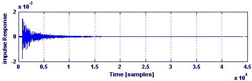
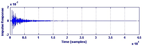
possible to generate an impulse response for that room. Using a simple tape measure we recorded
the height, width, and length of Duncan 1075 and a Will Rice dorm room, and used a MATLAB
program called Room Impulse Response to find the approximate impulse response of these two
rooms. We decided to take two samples in each room, leaving us with four theoretical impulse
responses.
<db:title>Theoretical Impulse in Duncan - Left</db:title> <db:title>Theoretical Impulse in Duncan - Right</db:title>
(b)
(a)
Figure 7.1.
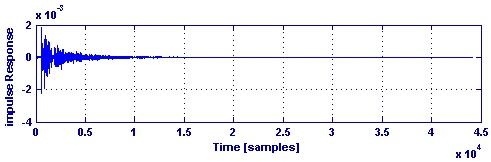
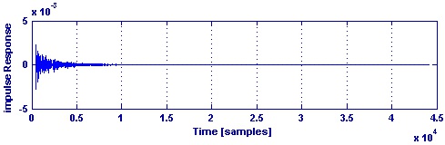
<db:title>Theoretical Impulse in Will Rice -
Left</db:title>
<db:title>Theoretical Impulse in
Will Rice - Right</db:title>
(b)
(a)
Figure 7.2.
Clearly these will not be incredibly accurate, as they assume a completely rectangular, and empty,
room. Neither of these rooms were completely rectangular, and they were also not empty.
However, this gives us a good approximation of the impulse response. The signals decay
significantly as time increases, which is expected. When we record the actual response using an
approximate impulse, this data will help determine if we have an accurate measurement.
Once we have the impulse response of each room, we must find an appropriate signal to
deconvolve. We chose a piano tune, as a piece of music should have a more simple frequency
response than speech. After recording the impulse response and the input, we theoretically have
enough data to reconstruct the signal using deconvolution. The recorded output is the convolution
of the input with the system. y ( t) = x ( t) * h ( t) The recorded output has a frequency spectrum defined by Y (jw) = X (jw) H (jw) Using simple algebra, we can solve for the input frequency coefficients: X (jw) = Y (jw) / H (jw) We have H(jw), the impulse response, and Y(jw), the FFT of the recorded signal. Thus we can find X(jw), the frequency spectrum of the input signal, and by
taking the inverse FFT we are left with the input signal x(t).
7.3. Recording the Impulse Response of a Room*
After obtaining the theoretical data we moved on to the measurements of the impulse response in
both rooms and audio test trials. The equipment that was used for the measurements was as
follows: a laptop computer, a pre amplifier, amplifier, speaker, and omnidirectional microphones.
The microphones and source were placed in accordance with the locations we specified in the
simulation software, given in rough estimate by the diagram.
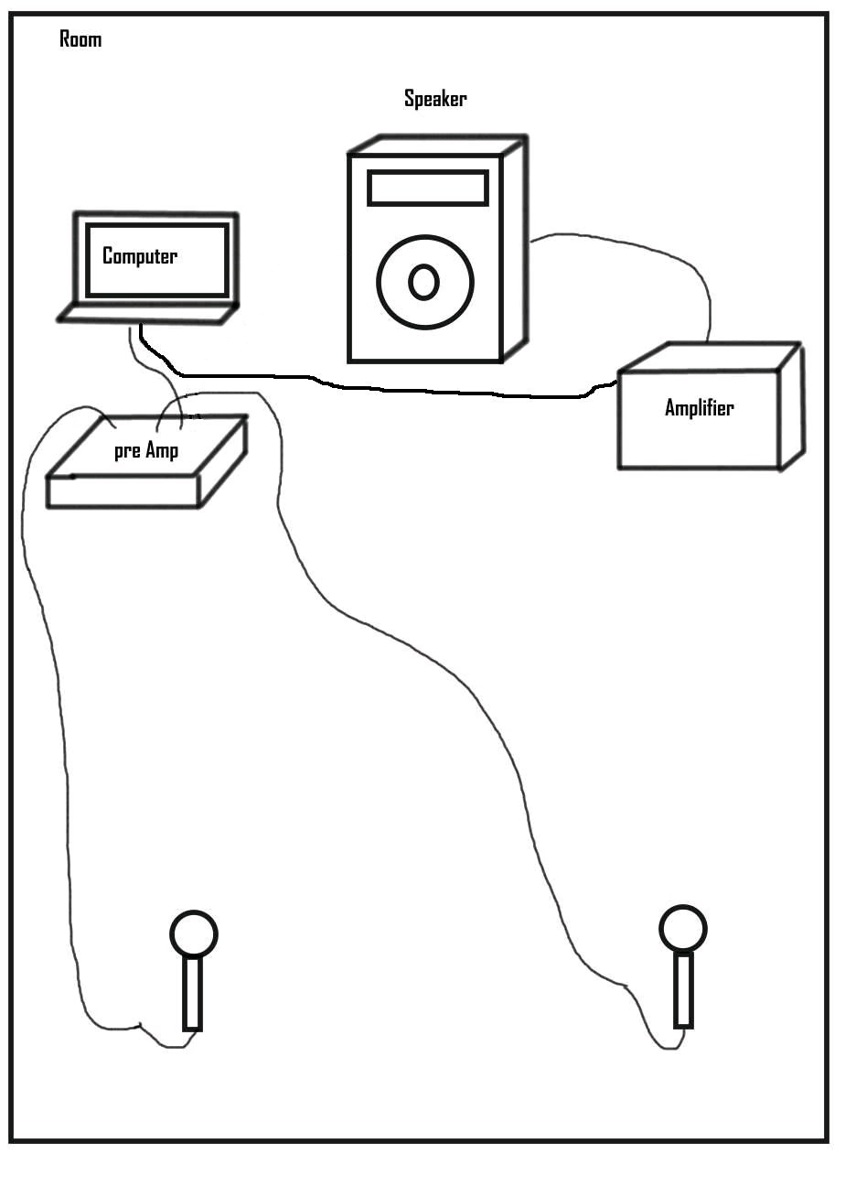
Figure 7.3. Recording Setup
The use of the laptop was necessary to not only record the test impulse response but as the source
of the impulse and test audio. To avoid the difficulty of making an impulse sound physically,
using a “clapper,” we generated an impulse digitally on the laptop with MATLAB. We used a
piano tune as the input hoping to become slightly more cultured while working on our project. In
order to properly record a significant number of reflections, very loud impulses and inputs were
played. This most likely resulted in clipping, but was necessary to determine accurate responses.
(This media type is not supported in this reader. Click to open media in browser.) (This
media type is not supported in this reader. Click to open media in browser.)
The impulse and input audio are used to perform the deconvolution experiment. The impulse and
the input signal were played in each of the rooms and the room responses to both of these were
recorded in .wav format. We recorded both responses in two rooms, Duncan 1075 and a Will Rice
College dorm room. We chose Duncan 1075 because it was the ELEC 301 classroom this year, and
a generic dorm room should help all of the audiophile students get the best sound quality possible.
We recorded two samples in each room, in case we found a null zone in one of the locations. The
results are displayed on the next page.
7.4. The Effectiveness of Naive Audio Deconvolution in a
Room*
After playing both the impulse responses and our input signal, and recording the output for two
points in each room, we were anxious to deconvolve our recorded input and get a perfect replica of
the input signal. All of our signals were recorded in .wav format, which is lossless, so we didn't
lose any important data due to audio compression. The results of our deconvolution in .wav format
are below.
(This media type is not supported in this reader. Click to open media in browser.)