

Statistical Mechanics by Konstantin K. Likharev - HTML preview
Download the book in PDF, ePub, Kindle for a complete version.
d
0
0
0
(3.62)
1 d()
N
2
d .
2 d
0
In the last form of this relation, the first integral over equals N( = 0) – N( = = 1, the second one vanishes (because the function under it is antisymmetric with respect to the point = ), and only the last one needs to be dealt with explicitly, by working it out by parts and then using a table integral:30
N
d
d
2
2
2
1
2
d T
d 4 2
T
4 2
T
(3.63)
d
0
e 1
0 e
1
12
Being plugged into Eq. (62), this result proves the Sommerfeld formula (59).
The last preparatory step we need to make is to account for a possible small difference (as we will see below, also proportional to T 2) between the temperature-dependent chemical potential ( T) and the Fermi energy defined as F (0), in the largest (first) term on the right-hand side of Eq. (59):
F
2 2 d()
2 2 d()
I T
( )
( ) d
. (3.64)
F ( )
T
I (0) F ()
T
6
d
6
d
0
Now, applying this formula to Eq. (41) and the last form of Eq. (52), we get the following results (which are valid for any dispersion law (p) and even any dimensionality of the gas): 2
dg
N( T) N( )
0 g
T
(3.65)
F
2
( )
( )
,
6
d
2
d
E( T ) E(0) g
T
g .
(3.66)
F
( )
2
( )
6
d
If the number of particles does not change with temperature, N( T) = N(0), as in most experiments, Eq.
(65) gives the following formula for finding the temperature-induced change of :
2 2 1 dg()
T
.
(3.67)
F
6
g() d
Note that the change is quadratic in T and negative, in agreement with the numerical results shown with the red line in Fig. 1. Plugging this expression (which is only valid when the magnitude of the change is much smaller than F) into Eq. (66), we get the following temperature correction to the energy: 30 See, e.g., MA Eqs. (6.8c) and (2.12b), with n = 1.
Chapter 3
Page 16 of 34
SM: Statistical Mechanics
2
2
E( T ) E( )
0
g() T ,
(3.68)
6
where within the accuracy of our approximation, may be replaced with F. (Due to the universal relation (48), this result also gives the temperature correction to the Fermi gas’ pressure.) Now we may use Eq. (68) to calculate the heat capacity of the degenerate Fermi gas:
Low-T
2
E
heat
C
T,
with
g
.
(3.69)
V
F
capacity
T
3
V
According to Eq. (55b), in the particular case of a 3D gas with the isotropic and parabolic dispersion law (3), Eq. (69) reduces to
2
2
N
CV
T
,
i.e. c
1.
(3.70)
2
V
N
2
F
F
This important result deserves a discussion. First, note that within the range of validity of the Sommerfeld approximation ( T << F), the specific heat of the degenerate gas is much smaller than that of the classical gas, even without internal degrees of freedom: cV = 3/2 – see Eq. (19). The physical reason for such a low heat capacity is that the particles deep inside the Fermi sea cannot pick up thermal excitations with available energies of the order of T << F, because the states immediately above them are already occupied. The only particles (or rather quantum states, due to the particle indistinguishability) that may be excited with such small energies are those at the Fermi surface, more exactly within a surface layer of thickness ~ T << F; Eq. (70) presents a very vivid manifestation of this fact.
The second important feature of Eqs. (69)-(70) is the linear dependence of the heat capacity on temperature, which decreases with a reduction of T much slower than that of crystal vibrations – see Eq.
(2.99). This means that in metals, the specific heat at temperatures T << T D is dominated by the conduction electrons. Indeed, experiments confirm not only the linear dependence (70) of the specific heat,31 but also the values of the proportionality coefficient CV/ T for cases when F can be calculated independently, for example for alkali metals – see the two rightmost columns of Table 1 above. More typically, Eq. (69) is used for the experimental measurement of the density of states on the Fermi surface, g(F) – the factor which participates in many theoretical results, in particular in transport properties of degenerate Fermi gases (see Chapter 6 below).
3.4. Bose-Einstein condensation
Now let us explore what happens at the cooling of an ideal gas of bosons. Figure 3a shows the same plot as Fig. 1b, i.e. the result of a numerical solution of Eq. (47) with the appropriate (lower) sign in the denominator, on a more appropriate log-log scale. One can see that the chemical potential
indeed tends to zero at some finite “critical temperature” T c. It may be found by taking = 0 in Eq. (47), thus reducing it to a table integral:32
31 Solids, with their low thermal expansion coefficients, provide virtually-fixed-volume confinement for the electron gas, so that the specific heat measured at ambient conditions may be legitimately compared with the calculated cV.
32 See, e.g., MA Eq. (6.8b) with s = 3/2, and then Eqs. (2.7b) and (6.7e).
Chapter 3
Page 17 of 34
SM: Statistical Mechanics
2
/ 3
2
/ 3
1/ 2
1
d
1
3 3
T T
T
313
.
3
T ,
(3.71) BEC:
c
0
0
0
2
2
critical
2
e 1
2
2 2
0
temperature
explaining the T c/ T 0 ratio which was already mentioned in Sec. 2 and indicated in Figs. 1 and 3.
(a)
(b)
100
10
8
PV NT
10
6
PV
3.313
)
NT
0
4
)
1
T 0
2
1.701
0
0.1
0
2
4
6
8
10
T / T 0
Fig. 3.3. The Bose-Einstein condensation:
(a) the chemical potential of the gas and (b)
0.01
1
10
100
its pressure, as functions of temperature. The
T / T
dashed line corresponds to the classical gas.
0
3.313
Let us have a good look at the temperature interval 0 < T < T c, which cannot be directly described by Eq. (40) (with the appropriate negative sign in the denominator), and hence may look rather mysterious. Indeed, within this range, the chemical potential cannot either be negative or equal to zero because according to Eq. (71); in this case, Eq. (40) would give a value of N smaller than the number of particles we actually have. On the other hand, cannot be positive either, because the integral (40) would diverge at due to the divergence of the factor N() – see, e.g., Fig. 2.15.
The only possible resolution of the paradox, suggested by A. Einstein in 1925, is as follows: at T
< T c, the chemical potential of each particle of the system still equals exactly zero, but a certain number ( N 0 of N) of them are in the ground state (with p 2/2 m = 0), forming the so-called Bose-Einstein condensate, usually referred to as the BEC. Since the condensate particles do not contribute to Eq. (40) (because of the factor 1/2 = 0), their number N 0 may be calculated by using that formula or, equivalently, Eq. (44) with = 0, to find the number ( N – N 0) of particles still remaining in the gas, i.e.
having energies > 0:
3 / 2
1/ 2
gV ( mT )
d
N N
.
(3.72)
0
2
3
2
0 e 1
Chapter 3
Page 18 of 34
SM: Statistical Mechanics
This result is even simpler than it may look. Indeed, let us write it for the case T = T c, when N 0 = 0:33
3 / 2
1/ 2
gV ( mT )
d
N
c
.
(3.73)
2
3
2
0 e
1
Dividing both sides of Eqs. (72) and (73), we get an extremely simple and elegant result: 3 / 2
3 / 2
N N
T
T
0
,
that
so
N N 1
, for T T .
(3.74a)
0
c
N
T
T
c
c
Please note that this result is only valid for the particles whose motion, within the volume V, is free – in other words, for a system of free particles confined within a rigid-wall box of volume V. In most experiments with the Bose-Einstein condensation of dilute gases of neutral (and hence very weakly interacting) atoms, they are held not in such a box, but at the bottom of a “soft” potential well, which may be well approximated by a 3D quadratic parabola: U(r) = m2 r 2/2. It is straightforward (and hence left for the reader’s exercise) to show that in this case, the dependence of N 0( T) is somewhat different: 3
T
N N 1
, for
*
T T ,
(3.74b)
0
*
c
T
c
where T *
c is a different critical temperature, which now depends on , i.e. on the confining potential’s
“steepness”. (In this case, V is not exactly fixed; however, the effective volume occupied by the particles at T = T *
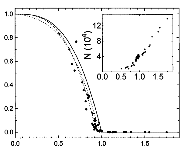
c is related to this temperature by a formula close to Eq. (71), so all estimates given above are still valid.) Figure 4 shows one of the first sets of experimental data for the Bose-Einstein condensation of a dilute gas of neutral atoms. Taking into account the finite number of particles in the experiment, the agreement with the simple theory is surprisingly good.
Returning to the spatially uniform Bose system, let us explore what happens below the critical temperature with its other parameters. Formula (52) with the appropriate (lower) sign shows that approaching T c from higher temperatures, the gas energy and hence its pressure do not vanish – see the red line in Fig. 3b. Indeed, at T = T c (where = 0), that formula yields34
3 / 2
5/2
3 / 2
3 / 2
5/2
m T
d
m T
5 5
c
c
E( T ) gV
gV
0.7701 NT ,
(3.75)
c
c
2
3
2
3
2
e 1
2
2 2
0
so using the universal relation (48), we get the following pressure value:
P T 2 E( T )
(5 / 2) N
N
c
T 0.5134
T 1.701 P ,
(3.76)
c
c
c
0
3 V
(3 / 2) V
V
which is somewhat lower than, but comparable with P(0) for the fermions – cf. Eq. (57).
33 This is, of course, just another form of Eq. (71). As was mentioned earlier, the dimensionless integral involved in all these three relations is equal to (3/2)(3/2) 2.315.
34 For the involved dimensionless integral see, e.g., MA Eqs. (6.8b) with s = 5/2, and then Eqs. (2.7b) and (6.7c).
Chapter 3
Page 19 of 34
Essential Graduate Physics
SM: Statistical Mechanics
Fig. 3.4. The total number N of trapped 87Rb
atoms (inset) and their ground-state fraction
N 0 /N, as functions of the ratio T/ T c, as measured N
in one of the pioneering experiments – see J.
0
Ensher et al., Phys. Rev. Lett. 77, 4984 (1996). In
N
this experiment, T *
c was as low as 0.2810-6 K.
The solid line shows the simple theoretical
dependence N( T) given by Eq. (74b), while other
lines correspond to more detailed theories taking
into account the finite number N of trapped
atoms. © 1996 APS, reproduced with permission.
*
T / T c
Now we can use the same Eq. (52), also with = 0, to calculate the energy of the gas at T < T c, 3 / 2
5 / 2
3 / 2
m T
d
E T gV
.
(3.77)
2
3
2
0 e 1
Comparing this relation with the first form of Eq. (75), which features the same integral, we immediately get one more simple temperature dependence:
5 / 2
T
E( T ) E T
, for T T .
(3.78) BEC:
c
c
T
energy
c
From the universal relation (48), we immediately see that the gas pressure follows the same dependence: 5 / 2
T
P( T ) P T
, for T T .
(3.79) BEC:
c
c
T
pressure
c
This temperature dependence of pressure is shown with the blue line in Fig. 3b. The plot shows that for all temperatures (both below and above T c) the pressure is lower than that of the classical gas of the same density. Now note also that since, according to Eqs. (57) and (76), P( T c) P 0 V-5/3, while according to Eqs. (35) and (71), T c T 0 V-2/3, the pressure (79) is proportional to V-5/3/( V-2/3)5/2 = V 0, i.e. does not depend on the volume at all! The physics of this result (which is valid at T < T c only) is that as we decrease the volume at a fixed total number N of particles, more and more of them go to the condensate, decreasing the number ( N – N 0) of particles in the gas phase, but not changing its spatial density and pressure. Such behavior is very typical for the coexistence of two different phases of the same matter – see, in particular, the next chapter.
The last thermodynamic variable of major interest is heat capacity, because it may be most readily measured. For temperatures T T c, it may be easily calculated from Eq. (78):
E
5 3/ 2
T
C ( T )
E( T )
,
(3.80)
V
c
T
2 5/2
T
N , V
c
so below T c, the capacity increases with temperature, at the critical temperature reaching the value Chapter 3
Page 20 of 34
SM: Statistical Mechanics
5 E( T )
C ( T )
c
1.925 N,
(3.81)
V
c
2 T c
which is approximately 28% above that (3 N/2) of the classical gas. (As a reminder, in both cases we ignore possible contributions from the internal degrees of freedom.) The analysis for T T c is a little bit more cumbersome because differentiating E over temperature – say, using Eq. (52) – one should also take into account the temperature dependence of that follows from Eq. (40) – see also Fig. 1.
However, the most important feature of the result may be predicted without such calculation (which is left for the reader’s exercise). Namely, since at T >> T c the heat capacity has to approach the classical value 1.5 N, a temperature increase from T c up must decrease CV from the value (81), thus forming a sharp maximum (a “cusp”) at the critical point T = T c – see Fig. 5.
3
3.313
2.5
2 1.925
CV
1.5
N
1
Fig. 3.5. Temperature dependences of the heat
0.5
capacity of an ideal Bose-Einstein gas,
numerically calculated from Eqs. (52) and (40)
0
0
2
4
6
8
10
for T T c, and given by Eq. (80) for T T c.
T / T
0
Such a cusp is a good indication of the Bose-Einstein condensation in virtually any experimental system, especially because inter-particle interactions (unaccounted for in our simple discussion) typically make this feature even more substantial, frequently turning it into a weak (logarithmic) singularity. Historically, such a singularity was the first noticed, though not immediately understood sign of the Bose-Einstein condensation observed in 1931 by W. Keesom and K. Clusius in liquid 4He at its - point (called so exactly because of the characteristic shape of the CV( T) plot) T = T c 2.17 K.
Other major milestones of the Bose-Einstein condensation research history include:
- the experimental discovery of superconductivity (which was later explained as the result of the Bose-Einstein condensation of electron pairs) by H. Kamerlingh-Onnes in 1911;
- the development of the Bose-Einstein statistics, and predicting the condensation, by S. Bose and A. Einstein, in 1924-1925;
- the discovery of superfluidity in liquid 4He by P. Kapitza and (independently) by J. Allen and D. Misener in 1937, and its explanation as a result of the Bose-Einstein condensation by F. and H.
Londons and L. Titza, with further significant elaborations by L. Landau – all in 1938;
- the explanation of superconductivity as a result of electron binding into Cooper pairs, with a simultaneous Bose-Einstein condensation of the resulting bosons, by J. Bardeen, L. Cooper, and J.
Schrieffer in 1957;
- the discovery of superfluidity of two different phases of 3He, due to the similar Bose-Einstein condensation of pairs of its fermion atoms, by D. Lee, D. Osheroff, and R. Richardson in 1972; Chapter 3
Page 21 of 34
SM: Statistical Mechanics
- the first observation of the Bose-Einstein condensation in dilute gases (87Ru by E. Cornell, C.
Wieman, et al. , and 23Na by W. Ketterle et al.) in 1995.
The importance of the last achievement stems from the fact that in contrast to other mentioned Bose-Einstein condensates, in dilute gases (with the typical density n as low as ~1014 cm-3) the particles interact very weakly, and hence many experimental results are very close to the simple theory described above and its straightforward elaborations – see, e.g., Fig. 4.35 On the other hand, the importance of other Bose-Einstein condensates, which involve more complex and challenging physics, should not be underestimated – as it sometimes is.
Perhaps the most important feature of any Bose-Einstein condensate is that all N 0 condensed particles are in the same quantum state, and hence are described by exactly the same wavefunction. This wavefunction is substantially less “feeble” than that of a single particle – in the following sense. In the second quantization language,36 the well-known commutation relations for the generalized coordinates and momenta may be rewritten for the creation/annihilation operators; in particular, for bosons,
ˆ a, ˆ†
a ˆ
I .
(3.82)
Since a ând †
ˆ a are the quantum-mechanical operators of the complex amplitude a = A exp{ i} and its complex conjugate a* = A exp{– i}, where A and are the real amplitude and phase of the wavefunction, Eq. (82) yields the following approximate uncertainty relation (strict in the limit << 1) between the number of particles N = AA* and the phase :
N
½ .
(3.83)
This means that a condensate of N >> 1 bosons may be in a state with both phase and amplitude of the wavefunction behaving virtually as c-numbers, with very small relative uncertainties: N << N,
<< 1. Moreover, such states are much less susceptible to unintentional perturbations including the instruments used for measurements. For example, the electric current carried along a superconducting wire by a coherent Bose-Einstein condensate of Cooper pairs may be as high as hundreds of amperes.
As a result, the “strange” behaviors predicted by the quantum mechanics are not averaged out as in the usual particle ensembles (see, e.g., the discussion of the density matrix in Sec. 2.1), but may be directly revealed in macroscopic, measurable dynamics of the condensate.
For example, the density j of the electric “supercurrent” of the Cooper pairs may be described by the same formula as the well-known usual probability current density of a single quantum particle,37 just multiplied by the electric charge q = –2 e of a single pair, and the pair density n:
q
j qn
A ,
(3.84)
m
35 Such controllability of theoretical description has motivated the use of dilute-gas BECs for modeling of renowned problems of many-body physics – see, e.g. the review by I. Bloch et al., Rev. Mod. Phys. 80, 885
(2008). These efforts are assisted by the development of better techniques for reaching the necessary sub-K
temperatures – see, e.g., the recent work by J. Hu et al., Science 358, 1078 (2017). For a more general, detailed discussion see, e.g., C. Pethick and H. Smith, Bose-Einstein Condensation in Dilute Gases, 2nd ed., Cambridge U.
Press, 2008.
36 See, e.g., QM Sec. 8.3.
37 See, e.g., QM Eq. (3.28).
Chapter 3
Page 22 of 34
SM: Statistical Mechanics
where A is the vector potential of the (electro)magnetic field. If a superconducting wire is not extremely thin, the supercurrent does not penetrate into its interior.38 As a result, the contour integral of Eq. (84), taken along a closed superconducting loop inside its interior (where j = 0), yields q
A d Δ 2 M
,
r
(3.85)
C
where M is an integer. But, according to the basic electrodynamics, the integral on the left-hand side of this relation is nothing more than the flux of the magnetic field B piercing the wire loop area A. Thus we immediately arrive at the famous magnetic flux quantization effect: 2
2
Φ
d r
Φ
M
,
Φ
where
B
2.07 10 15
Wb
,
(3.86)
n
0
0
q
A
which was theoretically predicted in 1950 and experimentally observed in 1961. Amazingly, this effect holds even (citing H. Casimir’s famous expression) “over miles of dirty lead wire”, sustained by the coherence of the Bose-Einstein condensate of Cooper pairs.
Other prominent examples of such macroscopic quantum effects in Bose-Einstein condensates include not only the superfluidity and superconductivity as such, but also the Josephson effect, quantized Abrikosov vortices, etc. Some of these effects are discussed in other parts of this series.39
3.5. Gases of weakly interacting particles
Now let us discuss the effects of weak particle interaction effects on the properties of their gas.
(Unfortunately, I will have time to do that only very briefly, and only for classical gases.40) In most cases of interest, particle interaction may be well described by a certain potential energy U, so in the simplest model, the total energy is
N
p 2
E k Ur ,.., r ,..., r ,
(3.87)
1
k
N
k 1 2 m
where r k is the radius vector of the k th particle’s center.41 First, let us see how far would the statistical physics allow us to proceed for an arbitrary potential U. For N >> 1, at the calculation of the Gibbs statistical sum (2.59), we may perform the usual transfer from the summation over all quantum states of the system to the integration over the 6 N-dimensional space, with the correct Boltzmann counting: N
N
/
1
g
p 2
(r ,... r )
Z E T
j
3
3
U
m
1
N
e
exp
d p d
...
p
exp
d 3 r d 3
... r
3
1
1
m
N! 2
N
N
N
k 1 2 mT
r V
T
k
38 This is the Meissner-Ochsenfeld (or just “Meissner”) effect which may be also readily explained using Eq. (84) combined with the Maxwell equations – see, e.g., EM Sec. 6.4.
39 See EM Secs. 6.4-6.5, and QM Secs. 1.6 and 3.1.
40 Discussions of the effects of weak interactions on the properties of quantum gases may be found, for example, in the textbooks by Huang and by Pathria and Beale – see References.
41 One of the most significant effects neglected by Eq. (87) is the influence of atomic/molecular angular orientations on their interactions.
Chapter 3
Page 23 of 34
SM: Statistical Mechanics
1
2
N
N
g V
N p
j
U r r N
3
3
1
( ,... )
1
3
3
d p d p
d r d r
(3.88)
N
N
N
N! 2
exp
...
exp
...
.
3
mT
N
k 1 2
1
1
V r V
T
k
But according to Eq. (14), the first operand in the last product is just the statistical sum of an ideal gas (with the same g, N, V, and T), so we may use Eq. (2.63) to write
1
U (r ,... r )
N
F F
T ln
exp
1
3
d r d r
N
... 3
ideal
1
N
V r V
T
k
(3.89)
1
F
T ln 1
U /
T
e
d r d r
ideal
N
1 3 ... 3 ,
1
N
V
r V
k
where F ideal is the free energy of the ideal gas (i.e. of the same gas but with U = 0), given by Eq. (16).
I believe that Eq. (89) is a very convincing demonstration of the enormous power of statistical physics methods. Instead of trying to solve an impossibly complex problem of classical dynamics of N
>> 1 (think of N ~ 1023) interacting particles, and only then calculating appropriate ensemble averages, the Gibbs approach reduces finding the free energy (and then, from thermodynamic relations, all other thermodynamic variables) to the calculation of just one integral on its right-hand side of Eq. (89). Still, this integral is 3 N-dimensional and may be worked out analytically only if the particle interactions are weak in some sense. Indeed, the last form of Eq. (89) makes it especially evident that if U 0
everywhere, the term in the parentheses under the integral vanishes, and so does the integral itself, and hence the addition to F ideal.
Now let us see what would this integral yield for the simplest, short-range interactions, in which the potential U is substantial only when the mutual distance r kk’ r k – r k’ between the centers of two particles is smaller than a certain value 2 r 0, where r 0 may be interpreted as the particle’s radius. If the gas is sufficiently dilute, so the radius r 0 is much smaller than the average distance r ave between the particles, the integral in the last form of Eq. (89) is of the order of (2 r 0)3 N, i.e. much smaller than ( r ave)3 N
VN. Then we may expand the logarithm in that expression into the Taylor series with respect to the small second term in the square brackets, and keep only its first non-zero term: T
F F
e
/
1 d 3 r d 3
... r .
(3.90)
ideal
N
U T 1
N
V r V
k
Moreover, if the gas density is so low, the chances for three or more particles to come close to each other and interact (collide) simultaneously are typically very small, so pair collisions are the most important ones. In this case, we may recast the integral in Eq. (90) as a sum of N( N – 1)/2 N 2/2 similar terms describing such pair interactions, each of the type
2
U
(r )/ T
N
kk
V
e
'
1
d 3 r d 3 r
.
(3.91)
k
k'
r , r V
k k '
It is convenient to think about the r kk’ r k – r k’ as the radius vector of the particle number k in the reference frame with the origin placed at the center of the particle number k’ – see Fig. 6a. Then in Eq.
(91), we may first calculate the integral over r k’, while keeping the distance vector r kk’, and hence U(r kk’), constant, getting one more factor V. Moreover, since all particle pairs are similar, in the remaining integral over r kk’ we may drop the radius vector’s index, so Eq. (90) becomes Chapter 3
Page 24 of 34


Essential Graduate Physics
SM: Statistical Mechanics
2
T N
N
U r T
T
1
( ) /
F F
V
e
d r F
N B T
(3.92)
ideal
N
1 3
2
( ),
V
2
ideal
V
where the function B( T), called the second virial coefficient,42 has an especially simple form for spherically symmetric interactions:
Second
1
r
3
1
virial
B T
( )
U ( ) / T
1 e
d r 4 r 2
dr
U( r)/ T
1 e
.
(3.93)
coefficient
2
2 0
From Eq. (92), and the second of the thermodynamic relations (1.35), we already know something particular about the equation of state P( V, T) of such a gas:
F
2
N T
2
N
N
P
P
B( T ) T
B( T )
.
(3.94)
ideal
2
2
V
V
V
V
T , N
We see that at a fixed gas density n = N/ V, the pair interaction creates additional pressure, proportional to ( N/ V)2 = n 2 and a function of temperature, B( T) T.
(a)
(b)
"
r
r r
"
r '
kk'
Fig. 3.6. The definition of the
particle k
'
r
interparticle distance vectors
at their (a) pair and (b) triple
interactions.
particle k’
Let us calculate B( T) for a few simple models of particle interactions. The solid curve in Fig. 7
shows (schematically) a typical form of the interaction potential between electrically neutral atoms/molecules. At large distances the interaction of particles without their own permanent electrical dipole moment p, is dominated by the attraction (the so-called London dispersion force) between the correlated components of the spontaneously induced dipole moments, giving U( r) r–6 at r .43 At closer distances the potential is repulsive, growing very fast at r 0, but its quantitative form is specific for particular atoms/molecules.44 The crudest description of such repulsion is given by the so-called hardball (or “hard-sphere”) model:
42 The term “virial”, from the Latin viris (meaning “force”), was introduced to molecular physics by R. Clausius.
The motivation for the adjective “second” for B( T) is evident from the last form of Eq. (94), with the “first virial coefficient”, standing before the N/ V ratio and sometimes denoted A( T), equal to 1 – see also Eq. (100) below.
43 Indeed, independent fluctuation-induced components p( t) and p ’( t) of dipole moments of two particles have random mutual orientation, so that the time average of their interaction energy, proportional to p( t)p ’( t)/ r 3, vanishes. However, the electric field E of each dipole p, proportional to r-3, induces a correlated component of p ’, also proportional to r-3, giving interaction energy U( r) proportional to p ’E r-6, with a non-zero statistical average. Quantitative discussions of this effect, within several models, may be found, for example, in QM
Chapters 3, 5, and 6.
44 Note that the particular form of the first term in the approximation U( r) = a/ r 12 – b/ r 6 (called either the Lennard-Jones potential or the “12-6 potential”), that had been suggested in 1924, lacks physical justification, and in professional physics was soon replaced with other approximations, including the so-called exp-6 model, Chapter 3
Page 25 of 34


Essential Graduate Physics
SM: Statistical Mechanics
,
0
for r 2 r ,
U ( r)
0
(3.95)
,
0
2
for
r r ,
0
– see the dashed line and the inset in Fig. 7. (The distance 2 r 0 is sometimes called the van der Waals radius of the particle.)
U ( r)
Fig. 3.7. Pair interactions of particles.
2 r 0
Solid line: a typical interaction potential;
dashed line: its hardball model (95);
0
r
dash-dotted line: the improved model
(97) – all schematically. The inset
U
min
illustrates the hardball model’s physics.
2 r 0
As Eq. (93) shows, in this model the second virial coefficient is temperature-independent: 2
1 0 r
2
4
2
B( T ) b
4 r
dr
2 r 4 V ,
where V
r
,
(3.96)
0 3
3
0
0
0
2
3
3
0
so the equation of state (94) still gives a linear dependence of pressure on temperature.
A correction to this result may be obtained by the following approximate account of the long-range attraction (see the dash-dotted line in Fig. 7):45
,
0
for r 2 r ,
U ( r)
0
(3.97)
U ( r) with
,
0
U T
2
for
,
r r .
0
For this improved model, Eq. (93) yields:
1
2
U ( r)
a
B( T ) b
4 r
dr
b ,
with a 2 U ( r) 2
r dr 0
.
(3.98)
2
T
T
2 0
r
2 0
r
In this model, the equation of state (94) acquires a temperature-independent term: 2
2
2
N
N
a
N
N
N
P T b T b a .
(3.99)
V V
T
V
V
V
Still, the correction to the ideal-gas pressure is proportional to ( N/ V)2 and has to be relatively small for this result to be valid.
which fits most experimental data much better. However, the Lennard-Jones potential still keeps creeping from one undergraduate textbook to another one, apparently for a not better reason than enabling a simple analytical calculation of the equilibrium distance between the particles at T 0.
45 The strong inequality U << T in this model is necessary not only to make the calculations simpler. A deeper reason is that if (– U min) becomes comparable with T, particles may become trapped in this potential well, forming a different phase – a liquid or a solid. In such phases, the probability of finding more than two particles interacting simultaneously is high, so Eq. (92), on which Eqs. (93)-(94) and Eqs. (98)-(99) are based, becomes invalid.
Chapter 3
Page 26 of 34
SM: Statistical Mechanics
Generally, the right-hand side of Eq. (99) may be considered as the sum of two leading terms in the general expansion of P into the Taylor series in low density n = N/ V of the gas: Pressure:
2
3
N
N
N
virial
P T B( T
)
C( T
)
... ,
(3.100)
expansion
V
V
V
where C( T) is called the third virial coefficient. It is natural to ask how can we calculate C( T) and the higher virial coefficients. This may be done by a tedious direct analysis of Eq. (90),46 but the calculations may be streamlined using a different, rather counter-intuitive approach called the cluster expansion method.47
Let us apply to our system, with the energy given by Eq. (87), the grand canonical distribution.
(Just as in Sec. 2, we may argue that if the average number N of particles in each member of a grand canonical ensemble, with fixed and T, is much larger than 1, the relative fluctuations of N are small, so all its thermodynamic properties should be similar to those when N is exactly fixed.) For our current purposes, Eq. (2.109) may be rewritten in the form
N
2
E
/ T
N T
p
T
ln Z , with
/
m, N
Z e
e
,
k
E
U ( r ,..., r ) .
(3.101)
N
N
m, N
N
N 0
m
k 2
1
1
m
(Notice that here, as at all discussions of the grand canonical distribution, N means a particular rather than the average number of particles.) Now let us try to forget for a minute that in real systems of interest the number of particles is extremely large, and start to calculate, one by one, the first terms ZN.
In the term with N = 0, both contributions to Em,N vanish, and so does the factor N/ T, and hence Z 0 = 1. In the next term, with N = 1, the interaction term vanishes, so Em,1 is reduced to the kinetic energy of one particle, giving
2
/ T
p
Z e
.
(3.102)
1
exp k
k
2 mT
Making the usual transition from the summation to integration, we may write
2
T
gV
p
Z ZI ,
where
/
3
Z e
d p
I .
(3.103)
1
1
2
exp
,
and
1
3
2
1
mT
This is the same simple (Gaussian) integral as in Eq. (6), giving
3 / 2
T
gV
T
mT
/
Z e
2 mT3/2
/
e
gV
.
(3.104)
2
3
2
2
Now let us explore the next term, with N = 2, which describes, in particular, pair interactions U =
U(r), with r = r – r ’. Due to the assumed particle indistinguishability, this term needs the “correct Boltzmann counting” factor 1/2! – cf. Eqs. (12) and (88):
46 L. Boltzmann has used that way to calculate the 3rd and 4th virial coefficients for the hardball model – as much as can be done analytically.
47 This method was developed in 1937-38 by J. Mayer and collaborators for the classical gas, and generalized to quantum systems in 1938 by B. Kahn and G. Uhlenbeck.
Chapter 3
Page 27 of 34
SM: Statistical Mechanics
1
2 /
p 2
p 2
Z
T
e
(r) /
exp
.
(3.105)
2
k k' U T
e
!
2 k, k' 2 mT 2 mT
Since U is coordinate-dependent, here the transfer from the summation to integration should be done more carefully than in the first term – cf. Eqs. (24) and (88):
2
2
2
2 / T 1 ( gV )
p
1
3
p'
Z e
3
U
(r)/ T 3
exp
exp
.
(3.106)
2
!
2 2
d p
d p'
e
d r
6
2 mT
2 mT
V
Comparing this expression with Eq. (103) for the parameter Z, we get
Z 2
1
Z
I ,
where I
e U (r)/ T d 3 r .
(3.107)
2
2
2
!
2
V
Acting absolutely similarly, for the third term of the grand canonical sum we may get Z 3
1
Z
I ,
where I
e U ( ' r, "
r ) / T d 3 r'd 3 r" ,
(3.108)
3
3
3
!
3
V 2
where r ’ and r ” are the vectors characterizing the mutual positions of three particles in their “cluster” –
see Fig. 6b.
These results may be readily generalized to clusters of arbitrary size N. Plugging the resulting expression for ZN into the first of Eqs. (101) and recalling that = – PV, we get the equation of state of the gas in the form
T
2
3
Z
Z
P
ln1 ZI
I
I ... .
(3.109)
1
2
3
V
!
2
!
3
As a sanity check: at U = 0, all integrals IN are equal to 1, and the expression under the logarithm is just the Taylor expansion of the function eZ, giving P = TZ/ V, and = – PV = – TZ. In this case, according to the last of Eqs. (1.62), the average number of particles in the system is N = –(/) T, V = Z, because since Z exp{/ T}, Z/ = Z/ T.48 Thus, in this limit, we have happily recovered the equation of state of the ideal gas.
Returning to the general case of non-zero interactions, let us assume that the logarithm in Eq.
(109) may be also represented as a direct Taylor expansion in Z:
T
J
Cluster
l
l
P
Z ,
(3.110) expansion:
V
pressure
l1 l!
where Jl are some Z-independent coefficients, still to be calculated. (The lower limit of the sum reflects the fact that according to Eq. (109), at Z = 0, P = ( T/ V) ln1 = 0, so the coefficient J 0 in a more complete version of Eq. (110) would equal 0 anyway.) According to Eq, (1.60), this expansion corresponds to the grand potential
J
l
l
PV T
Z .
(3.111)
l 1 l!
48 Actually, the fact that in that case N = Z could have been noted earlier – just by comparing Eq. (104) with Eq.
(32b).
Chapter 3
Page 28 of 34
SM: Statistical Mechanics
Again using the last of Eqs. (1.62), and the already mentioned fact that according to Eq. (104), Z/ =
Z/, we get
Cluster
J
expansion:
l
l
N
Z .
(3.112)
N
1 (
l
l
)!
1
(Note that this sum differs from that in Eq. (110) “only” by an extra factor l in each term.) Equations (110) and (112) essentially give the solution of our problem by representing the equation of state of the gas in the parametric form, with the factor Z serving as the parameter. The only remaining conceptual action item is to express the coefficients Jl via the integrals IN participating in the expansion (109). This may be done using the well-known Taylor expansion of the logarithm function, 49
l
ln 1
( )
l
1
1
.
(3.113)
l1
l
Applying it to Eq. (109), we get a Taylor series in Z, starting as
T
2
3
Z
Z
P
Z
( I )
1
I
I
.
(3.114)
2
( )1 (3 )1
3
2
...
V
!
2
!
3
Comparing this expression with Eq. (110), we see that
J ,
1
1
1
J I 1
U
(r)/
e
T d r
2
2
1 3 ,
V
(3.115)
J ( I )
1 (
3 I )
1
3
3
2
1
U
( '
r , "
r ) / T
U
( '
r ) / T
U
( "
r ) / T
U
( '''
r ) /
e
e
e
e
T d r'd r"
2
2 3
3
, ...
V
where ''
r ' '
r "
r – see Fig. 6b. The expression for J 2, describing the pair interactions of particles, shows that besides a factor of ( V/2), this is just the second virial coefficient B( T) – cf. Eq. (93). As a reminder, the subtraction of 1 from the integral I 2 in that expression makes the contribution of each elementary 3D volume d 3 r into the integral J 2 different from zero only if at this r two particles interact ( U 0). Very similarly, in the last of Eqs. (115), the subtraction of three pair-interaction terms from ( I 3
– 1) makes the contribution from an elementary 6D volume d 3 r’d 3 r” into the integral J 3 different from zero only if at that mutual location of particles, all three of them interact simultaneously, etc.
49 Looking at Eq. (109), one might think that since = Z + Z2 I 2/2 +… is of the order of at least Z ~ N, the expansion (113), which converges only if < 1, is illegitimate for N >> 1. However, it is justified by the result (114), in which the n th term is of the order of N n( V 0/ V) n-1/ n!, so that the series does converge if the gas density is sufficiently low: N/ V << 1/ V 0, i.e. r ave >> r 0. This is the very beauty of the cluster expansion whose few first terms, perhaps unexpectedly, give good approximation even for gases with N >> 1 particles. The physics behind this trick is that the subtraction of 1 from each exponent of the type exp{- U/ T} automatically includes, to the final result, contributions from only minor but the only important parts of the 6 N-dimensional phase space, in which the particles interact. As a result, the sum (114) is over the number of particles in each cluster (not in the whole gas!), with an analytical summation of equal contributions from all possible clusters with the same number l of particles in each of them – just as it is done by Eqs. (92)-(93) for the particular case l = 2.
Chapter 3
Page 29 of 34


Essential Graduate Physics
SM: Statistical Mechanics
The relations (110), (114), and (115) give the final result of the cluster expansion. To see this result at work, let us eliminate the factor Z from this system of equations, with accuracy up to terms O( Z 2). For that, we need to spell out each of these relations up to terms O( Z 3): PV
J
J
2
2
3
3
J Z
Z
Z ..., .
(3.116)
1
T
2
6
J
2
3
3
N J Z J Z
Z ... ,
(3.117)
1
2
2
and then divide these two expressions, getting the result
2
2
PV
1 ( J / 2 J ) Z ( J / 6 J ) Z ...
J
J
J
2
1
3
1
2
2
3
2
1
Z
Z .
(3.118)
2
2
N T
1 ( J / J ) Z ( J / 2 J ) Z ...
2 J
2 J
3 J
2
1
3
1
1
1
1
In this approximation, we may again use Eq. (117), now solved for Z with the same accuracy O( Z 2): J
2
2
Z N
N .
(3.119)
J 1
Plugging this expression into Eq. (118), we get the virial expansion (100) with 2
J
J
J
2nd and 3rd
2
2
3
2
B( T )
V ,
C( T )
V
.
(3.120) virial
2
2 J
J
3 J
1
1
1
coefficients
The first of these relations, combined with the first two of Eqs. (115), yields for the 2nd virial coefficient the same Eq. (93) that was obtained from the Gibbs distribution, in particular Eq. (96), B( T)
= 4 V 0, for the hardball model. The second of these results enables the calculation of the 3rd virial coefficient; for the hardball model, C( T) = 10 V 2
0 . (Let me leave the proof of the last result for the
reader’s exercise.) Evidently, a more complete expansion of Eqs. (110), (114), and (115) may be used to calculate an arbitrary virial coefficient, though starting from the 5th of them, the calculations of the necessary coefficients Jl may be completed only numerically even for the simplest hardball model.
Note that in this model, the virial coefficients B( T), C( T), etc. do not actually depend on temperature. (This is clear already from the above expressions for the integrals In and hence Jn.) As a result, by reproducing the calculations (1.45)-(1.47) for Eq. (100), we may readily see that the internal energy E of the gas, in the hardball model, is independent of its volume – just as for the ideal one.
3.6. Exercise problems
3.1. Use the Maxwell distribution for an alternative (statistical) calculation of the mechanical work performed by the Szilard engine discussed in Sec. 2.3.
Hint: You may assume the simplest geometry of the engine – see Fig. 2.4.
3.2. Use the Maxwell distribution to calculate the drag
A
coefficient –F/ u, where is the force exerted by an ideal classical gas on a piston moving with a low velocity u, in the simplest u
geometry shown in the figure on the right, assuming that collisions of
the gas particles with the piston are elastic.
Chapter 3
Page 30 of 34
SM: Statistical Mechanics
3.3. Derive the equation of state of an ideal classical gas from the grand canonical distribution.
3.4. Prove that Eq. (22), derived for the change of entropy at the mixing of two ideal classical gases of completely distinguishable particles (that initially had equal densities N/ V and temperatures T), is also valid if particles in each of the initial volumes are indistinguishable from each other but different from those in the counterpart volume. For simplicity, you may assume that the masses and internal degeneracy factors of all the particles are equal.
3.5. A round cylinder of radius R and length L, containing an ideal classical gas of N >> 1
particles of mass m each, is rotated about its symmetry axis with an angular velocity . Assuming that the gas as a whole rotates with the cylinder and is in thermal equilibrium at temperature T, (i) calculate the gas pressure distribution along the cylinder’s radius, and
(ii) neglecting the internal degrees of freedom of the particles, calculate the total energy of the gas and its heat capacity.
Analyze the results in the high- and low-temperature limits.
3.6. N >> 1 classical, non-interacting, indistinguishable particles of mass m are confined in a parabolic, spherically-symmetric 3D potential well U(r) = r 2/2. Use two different approaches to calculate all major thermodynamic characteristics of the system, including its heat capacity, in thermal equilibrium at temperature T. Which of the results should be changed if the particles are distinguishable?
Hint: Suggest a replacement of the notions of volume and pressure, appropriate for this system.
3.7. In the simplest model of thermodynamic equilibrium between the liquid and gas phases of the same molecules, temperature and pressure do not affect the molecule's condensation energy .
Calculate the density and pressure of such saturated vapor, assuming that it behaves as an ideal gas of classical particles.
3.8. An ideal classical gas of N >> 1 particles is confined in a container of volume V and wall surface area A. The particles may condense on the walls, releasing energy per particle and forming an ideal 2D gas on their surfaces. Calculate the number of condensed particles and the gas pressure, and discuss their temperature dependences, in thermodynamic equilibrium..
3.9. The inner surfaces of the walls of a closed container of volume V, filled with N >> 1
particles, have N S >> 1 similar particle traps (small potential wells). Each trap can hold only one particle, at a potential energy – < 0 relative to that in the volume. Assuming that the gas of the particles in the volume is ideal and classical, derive an equation for the chemical potential of the system in equilibrium, and use it to calculate this potential and the gas pressure in the limits of small and large values of the N/ N S ratio.
3.10. Calculate the magnetic response (the Pauli paramagnetism) of a degenerate ideal gas of spin-½ particles to a weak external magnetic field, due to a partial spin alignment with the field.
3.11. Calculate the magnetic response (the Landau diamagnetism) of a degenerate ideal gas of electrically charged fermions to a weak external magnetic field, due to their orbital motion.
Chapter 3
Page 31 of 34
SM: Statistical Mechanics
3.12.* Explore the Thomas-Fermi model of a heavy atom, with nuclear charge Q = Ze >> e, in which the electrons are treated as a degenerate Fermi gas, interacting with each other only via their contribution to the common electrostatic potential (r). In particular, derive the ordinary differential equation obeyed by the radial distribution of the potential, and use it to estimate the effective radius of the atom.50
3.13.* Use the Thomas-Fermi model that was explored in the previous problem to calculate the total binding energy of a heavy atom. Compare the result with that of a simpler model, in that the Coulomb electron-electron interaction is completely ignored.
3.14. Calculate the characteristic Thomas-Fermi length TF of weak electric field’s screening by conduction electrons in a metal, by modeling their ensemble as a degenerate, isotropic Fermi gas, with the electrons’ interaction limited (as in the two previous problems) by their contribution to the common electrostatic potential.
Hint: Assume that TF is much larger than the Bohr radius r B.
3.15. For a degenerate ideal 3D Fermi gas of N particles confined in a rigid-wall box of volume V, calculate the temperature effects on its pressure P and the heat capacity difference ( CP – CV), in the leading approximation in T << F. Compare the results with those for the ideal classical gas.
Hint: You may like to use the solution of Problem 1.9.
3.16. How would the Fermi statistics of an ideal gas affect the barometric formula (28)?
3.17. Derive general expressions for the energy E and the chemical potential of a uniform Fermi gas of N >> 1 non-interacting, indistinguishable, ultra-relativistic particles.51 Calculate E and also the gas pressure P explicitly in the degenerate gas limit T 0. In particular, is Eq. (48) valid in this case?
3.18. Use Eq. (49) to calculate the pressure of an ideal gas of ultra-relativistic, indistinguishable quantum particles, for an arbitrary temperature, as a function of the total energy E of the gas and its volume V. Compare the result with the corresponding relations for the electromagnetic blackbody radiation and for an ideal gas of non-relativistic particles.
3.19.* Calculate the speed of sound in an ideal gas of ultra-relativistic fermions of density n at negligible temperature.
50 Since this problem and the next one are important for atomic physics and, at their solution, thermal effects may be ignored, they were given in Chapter 8 of the QM part of the series as well, for the benefit of the readers who would not take this SM course. Note, however, that the argumentation in their solutions may be streamlined by using the notion of the chemical potential , which was introduced only in this course.
51 This is, for example, an approximate but reasonable model for electrons in a white dwarf star. (Their Coulomb interaction is mostly compensated by the electric charges of nuclei of fully ionized helium atoms.) Chapter 3
Page 32 of 34
SM: Statistical Mechanics
3.20. Calculate basic thermodynamic characteristics, including all relevant thermodynamic potentials, specific heat, and the surface tension of a non-relativistic 2D electron gas with a constant areal density n N/ A:
(i) at T = 0, and
(ii) at low temperatures (in the lowest nonvanishing order in T/F << 1), neglecting the Coulomb interaction effects.52
3.21. Calculate the differential latent heat ef ≡ – N( Q/ N 0) N,V of evaporation of a spatially uniform Bose-Einstein condensate as a function of temperature T. Here Q is the heat absorbed by the (condensate + gas) system of N >> 1 particles as a whole, while N 0 is the number of particles in the condensate alone.
3.22.* For a spatially uniform ideal Bose gas, calculate the law of the chemical potential’s disappearance at T T c and use the result to prove that at the critical point T = T c, the heat capacity CV
is a continuous function of temperature.
3.23. In Chapter 1, several thermodynamic relations involving entropy have been discussed, including the first of Eqs. (1.39):
S G
/ T
.
P
If we combine this expression with Eq. (1.56), G = N, it looks like that, for the Bose-Einstein condensate, the entropy should vanish because its chemical potential equals zero at temperatures below the critical point T c. On the other hand, by dividing both parts of Eq. (1.19) by dT, and assuming that at this temperature change the volume is kept constant, we get
C T S
T
V
/ . V
(This equality was also mentioned in Chapter 1.) If the CV is known as a function of temperature, the last relation may be integrated over T to calculate S:
C ( T )
S
V
dT
.
const
T
V const
According to Eq. (80), the specific heat for the Bose-Einstein condensate is proportional to T 3/2, so the integration gives a non-zero entropy S T 3/2. Resolve this apparent contradiction, and calculate the value of the genuine entropy at T = T c.
3.24. The standard analysis of the Bose-Einstein condensation, outlined in Sec. 4, may seem to ignore the energy quantization of the particles confined in volume V. Use the particular case of a cubic confining volume V = a a a with rigid walls to analyze whether the main conclusions of the standard theory, in particular Eq. (71) for the critical temperature of the system of N >> 1 particles, are affected by such quantization.
52 This condition may be approached reasonably well, for example, in 2D electron gases formed in semiconductor heterostructures (see, e.g., the discussion in QM Sec. 1.6, and the solution of Problem 3.2 of that course), due to not only the electron field’s compensation by background ionized atoms, but also by its screening by the highly doped semiconductor’s bulk.
Chapter 3
Page 33 of 34
SM: Statistical Mechanics
3.25.* N >> 1 non-interacting bosons are confined in a spherically symmetric potential well U(r)
= m2 r 2/2. Develop the theory of the Bose-Einstein condensation in this system; in particular, prove Eq.
(74b) and calculate the critical temperature T *
c . Looking at the solution, what is the most straightforward
way to detect the condensation in experiment?
3.26. Calculate the chemical potential of a uniform ideal 2D gas of spin-0 Bose particles as a function of its areal density n (the number of particles per unit area) , and find out whether such gas can condense at low temperatures. Review your result for the case of a large ( N >> 1) but finite number of particles.
3.27. Can the Bose-Einstein condensation be achieved in a 2D system of N >> 1 non-interacting bosons placed into the axially symmetric potential well U() = m22/2, where is the 2D radius vector
within the particle confinement plane? If yes, calculate the critical temperature of the condensation.
3.28. Use Eqs. (115) and (120) to calculate the third virial coefficient C( T) for the hardball model of particle interactions.
3.29. Assuming the hardball model, with volume V 0 per molecule, for the liquid phase, describe how the results of Problem 7 change if the liquid forms spherical drops of radius R >> V 1/3
0
. Briefly
discuss the implications of the result for water cloud formation in the atmosphere.
Hint: Surface effects in a macroscopic volume of a liquid may be well described by attributing an additional energy (equal to the surface tension) to the unit surface area.53
3.30. A 1D Tonks’ gas is a set of N classical hard rods of length l confined to a segment of length L > Nl, in thermal equilibrium at temperature T:
(i) Calculate the system’s average internal energy, entropy, both heat capacities, and the average force F exerted by the rods on the “walls” confining them to the segment L.
(ii) Expand the calculated equation of state F( L, T) into the Taylor series in linear density N/ L of the rods, find all virial coefficients, and compare the 2nd of them with the result following from the 1D
version of Eq. (93).
53 See, e.g., CM Sec. 8.2.
Chapter 3
Page 34 of 34
SM: Statistical Mechanics
Chapter 4. Phase Transitions
This chapter gives a brief discussion of the coexistence between different states (“phases”) of systems consisting of many similar interacting particles, and transitions between these phases. Due to the complexity of these phenomena, quantitative analytical results in this field have been obtained only for a few very simple models, typically giving rather approximate descriptions of real systems.
4.1. First-order phase transitions
From our everyday experience, say with water ice, liquid water, and water vapor, we know that one chemical substance (i.e. a system of many similar particles) may exist in different stable states –
phases. A typical substance may have:
(i) a dense solid phase, in which interparticle forces keep all atoms/molecules in virtually fixed relative positions, with just small thermal fluctuations about them;
(ii) a liquid phase, of comparable density, in which the relative distances between atoms or molecules are almost constant, but these particles are virtually free to move around each other, and (iii) a gas phase, typically of a much lower density, in which the molecules are virtually free to move all around the containing volume.1
Experience also tells us that at certain conditions, two different phases may be in thermal and chemical equilibrium – say, ice floating on water at the freezing-point temperature. Actually, in Sec. 3.4
we already discussed a quantitative theory of one such equilibrium: the Bose-Einstein condensate’s coexistence with the uncondensed gas of similar particles. However, this is a rather exceptional case when the phase coexistence is due to the quantum nature of the particles (bosons) rather than their direct interaction. Much more frequently, the formation of different phases and transitions between them are due to particle repulsive and attractive interactions, briefly discussed in Sec. 3.5.
Phase transitions are sometimes classified by their order.2 I will start their discussion with the so-called first-order phase transitions that feature non-zero latent heat – the thermal energy that is necessary to turn one phase into another phase completely, even if temperature and pressure are kept constant.3 Unfortunately, even the simplest “microscopic” models of particle interaction, such as those discussed in Sec. 3.5, give rather complex equations of state. (As a reminder, even the simplest hardball model leads to the series (3.100), whose higher virial coefficients defy analytical calculation.) This is 1 Plasma, in which atoms are partly or completely ionized, is frequently mentioned on one more phase, on equal footing with the three phases listed above, but one has to remember that in contrast to them, a typical electroneutral plasma consists of particles of two very different sorts – positive ions and electrons.
2 Such classification schemes, started by Paul Ehrenfest in the early 1930s, have been repeatedly modified to accommodate new results for particular systems, and by now only the “first-order phase transition” is still a generally accepted term, but with a definition different from the original one.
3 For example, for water the latent heat of vaporization at the ambient pressure is as high as ~2.2106 J/kg, i.e. ~
0.4 eV per molecule, making this ubiquitous liquid indispensable for fire fighting. (The latent heat of water ice’s melting is an order of magnitude lower.)
© K. Likharev
SM: Statistical Mechanics
why I will follow the tradition of discussing the first-order phase transitions on the example of a simple phenomenological model suggested in 1873 by Johannes Diderik van der Waals.
For its introduction, it is useful to recall that in Sec. 3.5 we have derived Eq. (3.99) – the equation of state for a classical gas of weakly interacting particles, which takes into account (albeit approximately) both interaction components necessary for a realistic description of gas condensation/liquefaction: the long-range attraction of the particles and their short-range repulsion. Let us rewrite that result as follows:
N 2
NT
Nb
P a
1
.
(4.1)
V 2
V
V
As we saw while deriving this formula, the physical meaning of the constant b is the effective volume of space taken by a particle pair collision – see Eq. (3.96). The relation (1) is quantitatively valid only if the second term in the parentheses is small, Nb << V, i.e. if the total volume excluded from particles’
free motion because of their collisions is much smaller than the whole volume V. In order to describe the condensed phase (which I will call “liquid” 4), we need to generalize this relation to the case Nb ~ V.
Since the effective volume left for particles’ motion is V – Nb, it is very natural to make the following replacement: V V – Nb, in the equation of state of the ideal gas.5 If we also keep on the left-hand side the term aN 2/ V 2, which describes the long-range attraction, we get the so-called van der Waals equation of state:
N 2
NT
Van der
P a
.
(4.2)
Waals
V 2
V Nb
equation
Taylor-expanding the right-hand side of this relation in small Nb/ V << 1, we see that its first two terms return us to the microscopically justified Eq. (1); however, already the next term of the expansion gives a virial coefficient C( T) different from the microscopically-derived Eq. (3.120), due to the phenomenological nature of Eq. (2). Let us explore the basic properties of this famous model.
It is frequently convenient to discuss any equation of state in terms of its isotherms, i.e. the P( V) curves plotted at constant T. As Eq. (2) shows, in the van der Waals model, such a plot depends on four parameters: a, b, N, and T, making formulas bulky. To simplify them, it is convenient to introduce dimensionless variables: pressure p P/ P c, volume v V/ V c, and temperature t T/ T c, all normalized to their so-called critical values,
1 a
8 a
P
, V 3 Nb, T
,
(4.3)
c
27 b 2
c
c
27 b
whose meaning will be clear in a minute. In this notation, Eq. (2) acquires the following form (historically called the law of corresponding states):
3
8 t
p
,
(4.4)
2
v
3 v 1
so the isotherms p( v) depend on only one parameter, the normalized temperature t – see Fig. 1.
4 Due to the phenomenological character of the van der Waals model, one cannot say for sure whether the condensed phase it predicts corresponds to a liquid or a solid. However, for most real substances at ambient conditions, gas coexists with liquid, hence the name.
5 For the 1D gas of non-zero-size particles (“rods”) with hard-core next-neighbor interactions, such replacement gives the exact result - see the solution of Problem 3.30. Unfortunately, this is not true in higher dimensions.
Chapter 4
Page 2 of 36
SM: Statistical Mechanics
2
2
.
1
1
.
1
P
p
P c
t 0
.
1
1
Fig. 4.1. The van der Waals equation of state,
9
.
0
plotted on the [ v, p] plane for several values of
the normalized temperature t T / T c. Shading
8
.
0
shows the range of single-phase instability
0
where ( P/ V)
0
1
2
T > 0.
v V / V c
The most important property of these plots is that the isotherms have qualitatively different shapes in two temperature regions. At t > 1, i.e. T > T c, pressure increases monotonically at gas compression (qualitatively, as in an ideal classical gas, with P = NT/ V, to which the van der Waals system tends at T >> T c), i.e. with ( P/ V) T < 0 at all points.6 However, below the critical temperature T c, any isotherm features a segment with ( P/ V) T >0. It is easy to understand that, at least in a constant-pressure experiment (see, for example, Fig. 1.5),7 these segments describe a mechanically unstable equilibrium. Indeed, if due to a random fluctuation, the volume deviated upward from its equilibrium value, the pressure would also increase, forcing the environment (say, the heavy piston in Fig. 1.5) to allow further expansion of the system, leading to an even higher pressure, etc. A similar deviation of volume downward would lead to a similar avalanche-like decrease. Such avalanche instability would develop further and further until the system has reached one of the stable branches with a negative slope ( P/ V) T. In the range where the single-phase equilibrium state is unstable, the system as a whole may be stable only if it consists of the two phases (one with a smaller, and another with a higher density n =
N/ V) that are described by the two stable branches – see Fig. 2.
P
stable liquid
phase
liquid and gas
in equilibrium
2'
A u
P ( T )
1
2
0
unstable
A
stable gaseous
d
branch
phase
Fig. 4.2. Phase equilibrium
'
1
0
at T < T
V
c (schematically).
6 The special choice of the numerical coefficients in Eq. (3) makes the border between these two regions take place exactly at t = 1, i.e. at the temperature equal to T c, with the critical point’s coordinates equal to P c and V c.
7 Actually, this assumption is not crucial for our analysis of mechanical stability, because if a fluctuation takes place in a small part of the total volume V, its other parts play the role of a pressure-fixing environment.
Chapter 4
Page 3 of 36
SM: Statistical Mechanics
In order to understand the basic properties of this two-phase system, let us recall the general conditions of the thermodynamic equilibrium of two systems, which have been discussed in Chapter 1: T T (thermal equilibrium),
(4.5)
1
2
(“chemical” equilibrium),
(4.6)
1
2
Phase
the latter condition meaning that the average energy of a single particle in both systems has to be the equilibrium conditions
same. To those, we should add the evident condition of mechanical equilibrium, P P (mechanical equilibrium),
(4.7)
1
2
which immediately follows from the balance of the normal forces exerted on any inter-phase boundary.
If we discuss isotherms, Eq. (5) is fulfilled automatically, while Eq. (7) means that the effective isotherm P( V) describing a two-phase system should be a horizontal line – see Fig. 2:8
P P ( T ) .
(4.8)
0
Along this line, the internal properties of each phase do not change; only the particle distribution is: it evolves gradually from all particles being in the liquid phase at point 1 to all particles being in the gas phase at point 2.9 In particular, according to Eq. (6), the chemical potentials of the phases should be equal at each point of the horizontal line (8). This fact enables us to find the line’s position: it has to connect points 1 and 2 in that the chemical potentials of the two phases are equal to each other. Let us recast this condition as
2
2
d ,0
i.e. dG 0 ,
(4.9)
1
1
where the integral may be taken along the single-phase isotherm. (For this mathematical calculation, the mechanical instability of states on a certain part of this curve is not important.) By definition, along that curve, N = const and T = const, so according to Eq. (1.53c), dG = – SdT + VdP + dN, for a slow (reversible) change, dG = VdP. Hence Eq. (9) yields
2
VdP 0.
(4.10)
1
This equality means that in Fig. 2, the shaded areas A d and A u should be equal. 10
8 Frequently, P 0( T) is called the saturated vapor pressure.
9 A natural question: is the two-phase state with P = P 0( T) the only state existing between points 1 and 2? Indeed, the branches 1-1 ’ and 2-2 ’ of the single-phase isotherm also have negative derivatives ( P/ V) T and hence are mechanically stable with respect to small perturbations. However, these branches are actually metastable, i.e.
have larger Gibbs energy per particle (i.e. ) than the counterpart phase at the same P, and are hence unstable to larger perturbations – such as foreign microparticles (say, dust), protrusions on the confining walls, etc. In very controlled conditions, these single-phase “superheated” and “supercooled” states can survive almost all the way to the zero-derivative points 1 ’ and 2 ’, leading to sudden jumps of the system into the counterpart phase. (At fixed pressure, such jumps go as shown by dashed lines in Fig. 2.) In particular, at the atmospheric pressure, purified water may be supercooled to almost –50C, and superheated to nearly +270C. However, at more realistic conditions, unavoidable perturbations result in the two-phase coexistence formation close to points 1 and 2.
10 This Maxwell equal-area rule (also called “Maxwell’s construct”) was suggested by J. C. Maxwell in 1875
using more complex reasoning.
Chapter 4
Page 4 of 36
SM: Statistical Mechanics
As the same Fig. 2 figure shows, the Maxwell rule may be rewritten in a different form, Maxwell
2
equal-area
P P ( T ) dV
0 ,
(4.11)
0
rule
1
which is more convenient for analytical calculations than Eq. (10) if the equation of state may be explicitly solved for P – as it is in the van der Waals model (2). Such calculation (left for the reader’s exercise) shows that for that model, the temperature dependence of the saturated vapor pressure at low T
is exponential,11
a
27
P ( T ) P exp
,
with
T , for T T ,
(4.12)
0
c
T
b
8 c
c
corresponding very well to the physical picture of the particle’s thermal activation from a potential well of depth .
The signature parameter of a first-order phase transition, the latent heat of evaporation 2
Latent
heat:
definition
dQ,
(4.13)
1
may also be found by a similar integration along the single-phase isotherm. Indeed, using Eq. (1.19), dQ
= TdS, we get
2
TdS T ( S S )
.
(4.14)
2
1
1
Let us express the right-hand side of Eq. (14) via the equation of state. For that, let us take the full derivative of both sides of Eq. (6) over temperature, considering the value of G = N for each phase as a function of P and T, and taking into account that according to Eq. (7), P 1 = P 2 = P 0( T):
G
G
dP
G
G
dP
1
1
0
2
2
0
.
(4.15)
T
P
dT T
P
dT
P
T
P
T
According to the first of Eqs. (1.39), the partial derivative ( G/ T) P is just minus the entropy, while according to the second of those equalities, ( G/ P) T is the volume. Thus Eq. (15) becomes dP
dP
S V
0 S V
0 .
(4.16)
1
1 dT
2
2 dT
Solving this equation for ( S 2 – S 1), and plugging the result into Eq. (14), we get the following Clapeyron-Clausius formula:
Clapeyron-
dP
Clausius
T V
(
V
0
)
.
(4.17)
2
1
formula
dT
For the van der Waals model, this formula may be readily used for the analytical calculation of in two limits: T << T c and ( T c – T) << T c – the exercises left for the reader. In the latter limit, ( T c – T)1/2, naturally vanishing at the critical temperature.
11 It is fascinating how well this Arrhenius exponent is hidden in the polynomial van der Waals equation (2)!
Chapter 4
Page 5 of 36
SM: Statistical Mechanics
Finally, some important properties of the van der Waals’ model may be revealed more easily by looking at the set of its isochores P = P( T) for V = const, rather than at the isotherms. Indeed, as Eq. (2) shows, all single-phase isochores are straight lines. However, if we interrupt these lines at the points when the single phase becomes metastable, and complement them with the (very nonlinear!) dependence P 0( T), we get the pattern (called the phase diagram) shown schematically in Fig. 3a.
(a)
(b)
P
V V
V V
c
c
P
critical
V V c
points
P
c
solid
liquid
liquid
gas
triple
point
P t
gas
0
T
0
T
c
T
t
T
Fig. 4.3. (a) Van der Waals model’s isochores, the saturated gas pressure diagram, and the critical point, and (b) the phase diagram of a typical three-phase system (all schematically).
In this plot, one more meaning of the critical point { P c, T c} becomes very vivid. At fixed pressure P < P c, the liquid and gaseous phases are clearly separated by the saturated pressure line P 0( T), so if we achieve the transition between the phases just by changing temperature (see the red horizontal arrow in Fig. 3a), we have to pass through the phase equilibrium point, being delayed there to either put the latent heat into the system or take it out. However, if we perform the transition between the same initial and final points by changing both the pressure and temperature in a way that we go around the critical point (see the blue arrow in Fig. 3a), no definite point of transition may be observed: the substance stays in a single phase, and it is a subjective judgment of the observer in which region that phase should be called the liquid, and in which region, the gas. For water, the critical point corresponds to the temperature of 647 K (374C), and the pressure P c 22.1 MPa (i.e. ~200 bars), so a lecture demonstration of its critical behavior would require substantial safety precautions. This is why such demonstrations are typically carried out with other substances such as either diethyl ether,12 with its much lower T c (194C) and P c (3.6 MPa), or the now-infamous carbon dioxide CO2, with even lower T c (31.1C), though higher P c (7.4 MPa). Though these substances are colorless and clear in both gas and liquid phases, their separation (by gravity) is still visible, due to small differences in the optical refraction coefficient, at P < P c, but not above P c.13
Thus, in the van der Waals model, two phases may coexist, though only at certain conditions – in particular, T < T c. Now a natural, more general question is whether the coexistence of more than two 12 (CH3-CH2)-O-(CH2-CH3), historically the first popular general anesthetic.
13 It is interesting that very close to the critical point the substance suddenly becomes opaque – in the case of ether, whitish. The qualitative explanation of this effect, called the critical opalescence, is simple: at this point, the difference of the Gibbs energies per particle (i.e. the chemical potentials) of the two phases becomes so small that unavoidable thermal fluctuations lead to spontaneous appearance and disappearance of relatively large (a-few-m-scale) single-phase regions in all the volume. A large concentration of boundaries of such randomly-shaped regions leads to strong light scattering.
Chapter 4
Page 6 of 36
SM: Statistical Mechanics
phases of the same substance is possible. For example, can the water ice, the liquid water, and the water vapor (steam) all be in thermodynamic equilibrium? The answer is essentially given by Eq. (6). From thermodynamics, we know that for a uniform system (i.e. a single phase), pressure and temperature completely define the chemical potential ( P, T). Hence, dealing with two phases, we had to satisfy just one chemical equilibrium condition (6) for two common arguments P and T. Evidently, this leaves us with one extra degree of freedom, so the two-phase equilibrium is possible within a certain range of P at fixed T (or vice versa) – see again the horizontal line in Fig. 2 and the bold line in Fig. 3a. Now, if we want three phases to be in equilibrium, we need to satisfy two equations for these variables:
( P, T ) ( P, T ) ( P, T ) .
(4.18)
1
2
3
Typically, the functions ( P, T) are monotonic, so the two equations (18) have just one solution, the so-called triple point { P t, T t}. Of course, this triple point of equilibrium between three phases should not be confused with the partial critical points { P c, T c} for each of the two-phase pairs. Fig. 3b shows, very schematically, their relation for a typical three-phase system solid-liquid-gas. For example, water, ice, and water vapor are at equilibrium at a triple point with P t 0.612 kPa14 and T t = 273.16 K. The practical importance of this particular temperature point is that by an international agreement, it has been accepted for the definition of not only the Kelvin temperature scale but also of the Celsius scale’s reference, as 0.01C, so the absolute temperature zero corresponds to exactly –273.15C.15 More generally, triple points of other purified simple substances (such as H2, N2, O2, Ar, Hg, and H2O) are also used for thermometer calibration, defining the so-called international temperature scales including the currently accepted scale ITS-90.
This analysis may be readily generalized to multi-component systems consisting of particles of several (say, L) sorts.16 If such a mixed system is in a single phase, i.e. is macroscopically uniform, its chemical potential may be defined by a natural generalization of Eq. (1.53c): L
l
l
dG SdT VdP dN .
(4.19)
l1
The last term reflects the fact that usually, every single phase is not a pure chemical substance, but has particles of all other components, so ( l) may depend not only on P and T but also on the concentrations c( l) N( l)/ N of particles of each sort. If the total number N of particles is fixed, the number of independent concentrations is ( L – 1). For the chemical equilibrium of R phases, all R values of ( l) r ( r =
1, 2, …, R) have to be equal for particles of each sort: ( l) ( l)
( l)
( l)
1 = 2 = … = R , with each r depending
on ( L – 1) concentrations c ( l)
r , and also on P and T. This requirement gives L( R – 1) equations for ( L –
1) R concentrations c ( l)
r , plus two common arguments P and T, i.e. for [( L –1) R + 2] independent variables. This means that the number of phases has to satisfy the limitation Gibbs
phase
L( R )
1 ( L )
1 R ,
2
i.e. R L 2 ,
(4.20)
rule
14 Please note that for water, P t is much lower than the normal atmospheric pressure (1 bar = 101.325 kPa).
15 Note the recent (2018) re-definition of the “legal” kelvin via joule (see, Appendix UCA: Selected Units and Constants); however, the new definition is compatible, within experimental accuracy, with that mentioned above.
16 Perhaps the most practically important example is the air/water system. For its detailed discussion, based on Eq.
(19), the reader may be referred, e.g., to Sec. 3.9 in F. Schwabl, Statistical Mechanics, Springer (2000). Other important applications include liquid solutions, and metallic alloys – solid solutions of metal elements.
Chapter 4
Page 7 of 36


Essential Graduate Physics
SM: Statistical Mechanics
where the equality sign may be reached at just one point in the whole parameter space. This is the Gibbs phase rule. As a sanity check, for a single-component system, L = 1, the rule yields R 3 – exactly the result we have already discussed.
4.2. Continuous phase transitions
As Fig. 2 illustrates, if we fix pressure P in a system with a first-order phase transition, and start changing its temperature, then the complete crossing of the transition-point line, defined by the equation P 0( T) = P, requires the insertion (or extraction) some non-zero latent heat . Formulas (14) and (17) show that is directly related to non-zero differences between the entropies and volumes of the two phases (at the same pressure). As we know from Chapter 1, both S and V may be represented as the first derivatives of appropriate thermodynamic potentials. This is why P. Ehrenfest called such transitions, involving jumps of potentials’ first derivatives, the first-order phase transitions.
On the other hand, there are phase transitions that have no first derivative jumps at the transition temperature T c, so the temperature point may be clearly marked, for example, by a jump of the second derivative of a thermodynamic potential – for example, the derivative C/ T which, according to Eq.
(1.24), equals to 2 E/ T 2. In the initial Ehrenfest classification, this was an example of a second-order phase transition. However, most features of such phase transitions are also pertinent to some systems in which the second derivatives of potentials are continuous as well. Due to this reason, I will use a more recent terminology (suggested in 1967 by M. Fisher), in which all phase transitions with = 0 are called continuous.
Most (though not all) continuous phase transitions result from particle interactions. Here are some representative examples:
(i) At temperatures above ~490 K, the crystal lattice of barium titanate (BaTiO3) is cubic, with a Ba ion in the center of each Ti-cornered cube (or vice versa) – see Fig. 4a. However, as the temperature is being lowered below that critical value, the sublattice of Ba ions is displaced along one of six sides of the TiO3 sublattice, leading to a small deformation of both lattices – which become tetragonal. This is a typical example of a structural transition, in this particular case combined with a ferroelectric transition, because (due to the positive electric charge of the Ba ions) below the critical temperature the BaTiO3 crystal has a spontaneous electric polarization even in the absence of external electric field.
(a)
(b)
Cu
Ba Ti O
Zn
Fig. 4.4. Single cells of
crystal lattices of (a)
BaTiO3 and (b) CuZn.
(ii) A different kind of phase transition happens, for example, in Cu x Zn1- x alloys (called brasses).
Their crystal lattice is always cubic, but above certain critical temperature T c (which depends on x) any of its nodes may be occupied by either a copper atom or a zinc atom, at random. At T < T c, a trend toward ordered atom alternation arises, and at low temperatures, the atoms are fully ordered, as shown in Fig. 4b for the stoichiometric case x = 0.5. This is a good example of an order-disorder transition.
Chapter 4
Page 8 of 36
SM: Statistical Mechanics
(iii) At ferromagnetic transitions (such as the one taking place, for example, in Fe at 1,388 K) and antiferromagnetic transitions (e.g., in MnO at 116 K), lowering of temperature below the critical value17 does not change atom positions substantially, but results in a partial ordering of atomic spins, eventually leading to their full ordering (Fig. 5).
(a)
(b)
Fig. 4.5. Classical images
of fully ordered phases: (a)
a ferromagnet, and (b) an
antiferromagnet.
Note that, as it follows from Eqs. (1.1)-(1.3), at ferroelectric transitions the role of pressure is played by the external electric field E, and at the ferromagnetic transitions, by the external magnetic field H. As we will see very soon, even in systems with continuous phase transitions, a gradual change of such an external field, at a fixed temperature, may induce jumps between metastable states, similar to those in systems with first-order phase transitions (see, e.g., the dashed arrows in Fig. 2), with non-zero decreases of the appropriate free energy.
Besides these standard examples, some other threshold phenomena, such as the formation of a coherent optical field in a laser, and even the self-excitation of oscillators with negative damping (see, e.g., CM Sec. 5.4), may be treated, at certain conditions, as continuous phase transitions.18
The general feature of all these transitions is the gradual formation, at T < T c, of certain ordering, which may be characterized by some order parameter 0. The simplest example of such an order parameter is the magnetization at the ferromagnetic transitions, and this is why continuous phase transitions are usually discussed for certain models of ferromagnetism. (I will follow this tradition but mention in passing other important cases that require a substantial modification of the theory.) Most of such models are defined on an infinite 3D cubic lattice (see, e.g., Fig. 5), with evident generalizations to lower dimensions. For example, the Heisenberg model of a ferromagnet (suggested in 1928) is defined by the following Hamiltonian:
Heisenberg
model
H ˆ J σˆ σˆ h σˆ ,
(4.21)
k
k '
k
k, k '
k
where
ˆ
ˆσ S / is the normalized Pauli vector operator19 acting on the quantum state of the k th spin, k
k
while h is the normalized external magnetic field B:
17 For ferromagnets, this point is usually referred to at the Curie temperature, and for antiferromagnets, as the Néel temperature.
18 Unfortunately, I will have no time/space for these interesting (and practically important) generalizations, and have to refer the interested reader to the famous monograph by R. Stratonovich, Topics in the Theory of Random Noise, in 2 vols., Gordon and Breach, 1963 and 1967, and/or the influential review by H. Haken, Ferstkörperprobleme 10, 351 (1970).
Chapter 4
Page 9 of 36
SM: Statistical Mechanics
h
B
.
(4.22)
(Here is the gyromagnetic ratio of the particle; for an electron, is very close to – e/ m e, so the effective magnitude m0 = / 2 of the spin’s magnetic moment is very close to the Bohr magneton B e/2 m e
0.92710-23 J/T.) The figure brackets { k, k’} in Eq. (21) denote the summation over the pairs of adjacent lattice sites, so the magnitude of the constant J may be interpreted as the maximum coupling energy per
“bond” between two adjacent particles. At J > 0, the coupling tries to keep spins aligned, i.e. to install the ferromagnetic ordering.20 The second term in Eq. (21) describes the effect of the external magnetic field, which tries to orient all spin magnetic moments along its direction.21
However, even the Heisenberg model, while being rather rudimentary (in particular because its standard form (21) is only valid for spins-½), is still rather complex for analysis. This is why most theoretical results have been obtained for its classical twin, the Ising model:22
E J
s s
h
s .
(4.23) Ising
m
k k '
k
model
k, k '
k
Here Em are the particular values of the system’s energy in each of its 2 N possible states with all possible combinations of the binary classical variables sk = 1, while h is the normalized external magnetic field’s magnitude – see Eq. (22). (Despite its classical character, the variable sk, modeling the field-oriented Cartesian component of the real spin, is usually called “spin” for brevity, and I will follow this tradition.) Somewhat shockingly, even for this toy model, no exact analytical 3D solution that would be valid at arbitrary temperatures has been found yet, and the solution of its 2D version by L. Onsager in 1944 (see Sec. 5 below) is still considered one of the top intellectual achievements of statistical physics.
Still, Eq. (23) is very useful for the introduction of the basic notions of continuous phase transitions and methods of their analysis, so for my brief discussion, I will mostly use this model.23
Evidently, if T = 0 and h = 0, the lowest possible energy,
E
JNd ,
(4.24)
min
where d is the lattice dimensionality, is achieved in the “ferromagnetic” phase in which all spins sk are equal to either +1 or –1, so sk = 1 as well. On the other hand, at J = 0, the spins are independent, and if h = 0 as well, all sk are completely random, with a 50% probability to take either of values 1, so sk
= 0. Hence in the general case (with arbitrary J and h), we may use the average Ising
s
(4.25) model:
k
order
parameter
19 See, e.g., QM Sec. 4.4.
20 At J < 0, the first term of Eq. (21) gives a reasonable model of an antiferromagnet, but in this case, the external magnetic field effects are more subtle; I will not have time to discuss them.
21 See, e.g., QM Eq. (4.163).
22 Named after Ernst Ising who explored the 1D version of the model in detail in 1925, though a similar model was discussed earlier (in 1920) by Wilhelm Lenz.
23 For more detailed discussions of phase transition theories (including other popular models of the ferromagnetic phase transition, e.g., the Potts model), see, e.g., either H. Stanley, Introduction to Phase Transitions and Critical Phenomena, Oxford U. Press, 1971; or A. Patashinskii and V. Pokrovskii, Fluctuation Theory of Phase Transitions, Pergamon, 1979; or B. McCoy, Advanced Statistical Mechanics, Oxford U. Press, 2010. For a very concise text, I can recommend J. Yeomans, Statistical Mechanics of Phase Transitions, Clarendon, 1992.
Chapter 4
Page 10 of 36
SM: Statistical Mechanics
as a good measure of spin ordering, i.e. as the order parameter. Since in a real ferromagnet, each spin carries a magnetic moment, the order parameter is proportional to the Cartesian component of the system’s average magnetization, in the direction of the applied magnetic field.
Now that the Ising model has given us a very clear illustration of the order parameter, let me use this notion for a semi-quantitative characterization of continuous phase transitions. Due to the difficulty of theoretical analyses of most models of the transitions at arbitrary temperatures, their theoretical discussions are focused mostly on a very close vicinity of the critical point T c. Both experiment and theory show that in the absence of an external field, the function ( T) is close to a certain power,