

Quantum Mechanics by Konstantin K. Likharev - HTML preview
Download the book in PDF, ePub, Kindle for a complete version.
B
2
thermal
2
2
equilibrium
This is a very interesting result: the density matrix depends only on the difference of its arguments, dropping to zero fast as the distance between the points x and x’ exceeds the following characteristic scale (sometimes called the correlation length or correlation distance 17) 1/ 2
x x x' 2
(7.37) Correlation
c
length
mk T
B
.
1/ 2
Some gut feeling of this length may be obtained from the following observation. It is straightforward to use Eq. (24) to verify that the average energy E = p 2/2 m of a free particle in thermal equilibrium, i.e.
in the classical mixture (33), equals k B T/2. (This value agrees with the equipartition theorem of classical statistics.18) Hence the average magnitude of the particle’s momentum may be estimated as 1/ 2
2
p p
m E
mk T
(7.38)
c
2
1/2 B 1/2,
so x c is of the order of the minimal length allowed by the Heisenberg-like “uncertainty relation”: x
.
(7.39)
c
p c
With the growth of temperature, the correlation length (37) goes to zero, and the density matrix (36) tends to a delta function:
(
w x, x' ) Z
( x x' )
T
.
(7.40)
Since in this limit the average kinetic energy of the particle is not smaller than its potential energy in any fixed potential profile, Eq. (40) is the general property of the density matrix (33).
16 Due to the delta-normalization of the eigenfunction, the density matrix (34) for the free particle (and any system with a continuous eigenvalue spectrum) is normalized as
(
w x, x' ) Zdx'
(
w x, x' ) Zdx .
1
17 Note that in some other fields of physics, the same term is used for a differently defined notion – see, e.g., SM
Eqs. (4.30)-(4.31).
18 See, e.g., SM Sec. 2.2.
Chapter 7
Page 8 of 54
QM: Quantum Mechanics
Moreover, as will be shown in a minute (see Eq. (61) below), Eq. (36) may be used to calculate not only the r.m.s. magnitude p c of the free particle’s momentum19 but also the whole distribution of the momentum’s probability density. Thus for mixed states, the density function w( x, x’) is indeed much more informative than the probability distribution w( x) – which, in our current case, is flat.
Now note the following important feature of Eq. (36): if we replace k B T with / i( t – t 0), and x’
with x 0, the un-normalized density matrix wZ for a free particle turns into the particle’s propagator – cf.
Eq. (2.49). This is not just an occasional coincidence. Indeed, in Chapter 2 we saw that the propagator of a system with an arbitrary stationary Hamiltonian may be expressed via the stationary eigenfunctions as
En
*
G( x, t; x , t )
0
0
( x)exp i
t t
( x )
n
0 n 0 .
(7.41)
n
Comparing this expression with Eq. (33), we see that the replacement
i( t t )
0
1
,
(7.42)
k T
B
plus the notation replacement x’ x 0, turn the pure-state propagator G into the un-normalized density matrix wZ of the same system in thermodynamic equilibrium. This important fact, rooted in the mathematical similarity of the Gibbs distribution (24) with the Schrödinger equation’s solution (1.69), enables a theoretical technique of the so-called thermodynamic Green’s functions, which is especially productive in condensed matter physics.20
For our current purposes, we can employ Eq. (42) to reuse some of the wave mechanics results, in particular, the following formula for the harmonic oscillator’s propagator
m
1/2
m x
x
t t
xx
0
0
2 20cos[ ( )]2
0
0
0
G( x, t; x , t )
. (7.43)
0
0
exp
2 i
sin[ ( t t )]
i
t t
0
0
2 sin[
( )]
0
0
which may be readily proved to satisfy the Schrödinger equation for the Hamiltonian (5.62), with the appropriate initial condition: G( x, t 0; x 0, t 0) = ( x – x 0). Making the substitution (42), we immediately get Harmonic
1/ 2
oscillator
m
m x x'
k T xx'
0
0
2 2cosh /0 B 2
(
w x, x') Z
in thermal
(7.44)
2
equilibrium
sinh
k T
k T
0
B
exp
/
2 sinh
0 B
.
/
As a sanity check, at very low temperatures, k B T << 0, both hyperbolic functions participating in this expression are very large and nearly equal, and it yields
m
m x
m
m x'
0 1/ 4
2
1/ 4
0
0
0
2
(
w x, x' ) Z
0
T
exp
0
exp
exp
. (7.45)
2 k T
B
19 This is what could be expected from the basic equation (5): the density matrix enables the calculation of the statistical average of any variable pertaining to the system – including its momentum.
20 I will have no time to discuss this technique and have to refer the interested reader to special literature.
Probably, the most famous text of that field is A. Abrikosov, L. Gor’kov, and I. Dzyaloshinski, Methods of Quantum Field Theory in Statistical Physics, Prentice-Hall, 1963. (Later reprintings are available from Dover.) Chapter 7
Page 9 of 54
QM: Quantum Mechanics
In each of the expressions in square brackets, we can readily recognize the ground state’s wavefunction (2.275) of the oscillator, while the middle exponent is just the statistical sum (24) in the low-temperature limit when it is dominated by the ground-level contribution:
Z
0
T
exp
0
.
(7.46)
2 k T
B
As a result, Z in both parts of Eq. (45) may be canceled, and the density matrix in this limit is described by Eq. (31), with the ground state as the only state of the oscillator. This is natural when the temperature is too low for the thermal excitation of any other state.
Returning to arbitrary temperatures, Eq. (44) in coinciding arguments gives the following expression for the probability density:21
1/ 2
2
m
m x
(
w x, x) Z (
w x)
0
0
0
Z
(7.47)
2sinh
/ k T
k T
0
B
exp
tanh
.
2
B
This is just a Gaussian function of x, with the following variance:
x 2
0
coth
.
(7.48)
2 m
2 k T
0
B
To compare this result with our earlier ones, it is useful to recast it as
2
m
0
2
0
U
x
coth
0 .
(7.49)
2
4
2 k T
B
Comparing this expression with Eq. (26), we see that the average value of potential energy is exactly one-half of the total energy – the other half being the average kinetic energy. This is what we could expect, because according to Eqs. (5.96)-(5.97), such relation holds for each Fock state and hence should also hold for their classical mixture.
Unfortunately, besides the trivial case (30) of coinciding arguments, it is hard to give a straightforward interpretation of the density function in terms of the system’s measurements. This is a fundamental difficulty, which has been well explored in terms of the Wigner function (sometimes called the “Wigner-Ville distribution”)22 defined as
~
~
~
1
X
X
iPX ~
Wigner
W ( X , P)
w X
, X
exp
dX .
(7.50) function:
2
2
2
definition
From the mathematical standpoint, this is just the Fourier transform of the density matrix in one of two new coordinates defined by the following relations (see Fig. 2):
21 I have to confess that this notation is imperfect, because strictly speaking, w( x, x’) and w( x) are different functions, and so are the functions w( p, p’) and w( p) used below. In a perfect world, I would use different letters for them all, but I desperately want to stay with “w” for all the probability densities, and there are not so many good fonts for this letter. Let me hope that the difference between these functions is clear from their arguments and the context.
22 It was introduced in 1932 by Eugene Wigner on the basis of a general ( Weyl-Wigner) transform suggested by Hermann Weyl in 1927 and re-derived in 1948 by Jean Ville on a different mathematical basis.
Chapter 7
Page 10 of 54
QM: Quantum Mechanics
~
~
x x'
~
X
X
X
, X x x',
that
so
x X
, x' X
.
(7.51)
2
2
2
Physically, the new argument X may be interpreted as the average position of the particle during
~
the time interval ( t – t’), while X , as the distance passed by it during that time interval, so P
characterizes the momentum of the particle during that motion. As a result, the Wigner function may be understood as a mathematical construct intended to characterize the system’s probability distribution simultaneously in the coordinate and the momentum space – for 1D systems, on the phase plane [ X, P]
that was discussed earlier – see Fig. 5.8. Let us see how fruitful this intention is.
x'
X 2
~
x
Fig. 7.2. The coordinates X and X employed in the Weyl-
0
Wigner transform (50). They differ from the coordinates
~
X
obtained by the rotation of the reference frame by the angle
/4 only by factors 2 and 1/2, describing scale stretch.
2
First of all, we may write the Fourier transform reciprocal to Eq. (50):
~
~
~
X
X
iPX
w X
, X
W ( X , P) exp
dP
.
(7.52)
2
2
~
For the particular case X 0 , this relation yields
w( X ) w( X , X ) W( X, P) dP .
(7.53)
Hence the integral of the Wigner function over the momentum P gives the probability density to find the system at point X – just as it does for a classical distribution function w cl( X, P).23
Next, the Wigner function has a similar property for its integration over X. To prove this fact, we may first introduce the momentum representation of the density matrix, in full analogy with its coordinate representation (27):
w( p, p' ) p ˆ w p' .
(7.54)
Inserting, as usual, two identity operators, in the form given by Eq. (4.252), into the right-hand side of this equality, we get the following relation between the momentum and coordinate representations: 1
ipx
ip'x'
w( p, p' )
dxdx' p x x w ˆ x' x' p'
dxdx' exp w( x, x' )exp
. (7.55)
2
This is of course nothing else than the unitary transform of an operator from the x-basis to the p-basis, similar to the first form of Eq. (4.272). For coinciding arguments, p = p’, Eq. (55) is reduced to 23 Such function, used to express the probability dW to find the system in a small area of the phase plane as dW = w cl( X, P) dXdP, is a major notion of the (1D) classical statistics – see, e.g., SM Sec. 2.1.
Chapter 7
Page 11 of 54
QM: Quantum Mechanics
1
ip( x x' )
(
w p) (
w p, p)
dxdx' (
w x, x' ) exp
.
(7.56)
2
Now using Eq. (29) and then Eq. (4.265), this function may be represented as
1
*
ip( x x' )
w( p)
W dxdx' ( x) ( x)exp
W
*
,
(7.57)
j
j
j
j
j p
j p
2 j
j
and hence interpreted as the probability density of the particle’s momentum at value p. Now, in the variables (51), Eq. (56) has the form
~
~
~
1
X
X
ipX ~
(
w p)
w X
, X
exp
dXdX .
(7.58)
2
2
2
Comparing this equality with the definition (50) of the Wigner function, we see that w( P) W( X, P) dX .
(7.59)
Thus, according to Eqs. (53) and (59), the integrals of the Wigner function over either the coordinate or momentum give the probability densities to find the system at a certain value of the counterpart variable. This is of course the main requirement for any quantum-mechanical candidate for the best analog of the classical probability density, w cl( X, P).
Let us see how the Wigner function looks for the simplest systems at thermodynamic equilibrium. For a free 1D particle, we can use Eq. (34), ignoring for simplicity the normalization issues:
~ 2
~
mk TX
iPX
B
~
W ( X , P) exp
exp
X
d .
(7.60)
2 2
The usual Gaussian integration yields
P 2
W ( X , P) const exp
.
(7.61)
2 mk T
B
We see that the function is independent of X (as it should be for this translational-invariant system), and coincides with the Gibbs distribution (24).24 We could get the same result directly from classical statistics. This is natural because as we know from Sec. 2.2, the free motion is essentially not quantized
– at least in terms of its energy and momentum.
Now let us consider a “more quantum” system, the harmonic oscillator. Plugging Eq. (44) into Eq. (50), for that system in thermal equilibrium it is easy (and hence is left for the reader’s exercise) to show that the Wigner function is also Gaussian, now in both its arguments:
2
2
2
m X
P
W ( X , P) const exp
0
C
,
(7.62)
2
2
m
though the coefficient C is now different from 1/ k B T, and tends to that limit only at high temperatures,
k B T >> 0. Moreover, for a Glauber state, the Wigner function also gives a very vivid result – a 24 Note also that the width of this Gaussian distribution of momentum is indeed given by Eq. (38).
Chapter 7
Page 12 of 54
Essential Graduate Physics
QM: Quantum Mechanics
Gaussian distribution similar to Eq. (62), but properly shifted from the origin to the central point of the state – see Sec. 5.5.
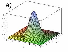
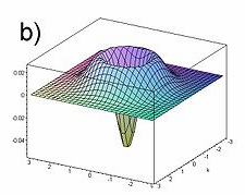
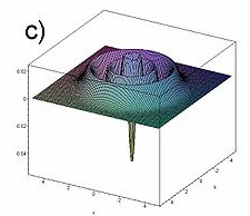
However, for some other possible states of the harmonic oscillator, e.g., any pure Fock state with n > 0, the Wigner function takes negative values in some regions of the [ X, P] plane – see Fig. 3.25 (Such plots were the basis of my, admittedly very imperfect, classical images of the Fock states in Fig. 5.8.) Fig. 7.3. The Wigner functions W( X, P) of a harmonic oscillator, in a few of its stationary (Fock) states n: (a) n = 0, (b) n = 1; (c) n = 5. Graphics by J. S. Lundeen; adapted from http://en.wikipedia.org/wiki/Wigner_function as a public-domain material.
The same is true for most other quantum systems and their states. Indeed, this fact could be predicted just by looking at the definition (50) applied to a pure quantum state, in which the density function may be factored – see Eq. (31):
~
~
~
1
X *
X
iPX ~
W ( X , P)
X
X exp
dX .
(7.63)
2
2
2
By changing the argument P (say, at fixed X), we are essentially changing the spatial “frequency” (wave number) of the wavefunction product’s Fourier component we are calculating, and we know that their Fourier images typically change sign as the frequency is changed. Hence the wavefunctions should have some high-symmetry properties to avoid this effect. Indeed, the Gaussian functions (describing, for example, the Glauber states, the squeezed states, and in their particular case, the ground state of the harmonic oscillator) have such symmetry, but many other functions do not.
Hence the Wigner function cannot serve as a direct quantum-mechanical analog of the classical probability density w cl( X, P). However, the function is useful for semi-quantitative interpretation of complicated mixed states of quantum systems.
7.3. Open system dynamics: Dephasing
So far we have discussed the density operator as something given at a particular time instant.
Now let us discuss how is it formed, i.e. its evolution in time, starting from the simplest case when the probabilities Wj participating in Eq. (15) are time-independent – by this or that reason, to be discussed in a moment. In this case, in the Schrödinger picture, we may rewrite Eq. (15) as
25 Spectacular experimental measurements of this function (for n = 0 and n = 1) were carried out recently by E.
Bimbard et al., Phys. Rev. Lett. 112, 033601 (2014).
Chapter 7
Page 13 of 54
QM: Quantum Mechanics
w ˆ t
( ) w t() W w t() .
(7.64)
j
j
j
j
Taking a time derivative of both sides of this equation, multiplying them by i, and applying Eq. (4.158) to the basis states wj, with the account of the fact that the Hamiltonian operator is Hermitian, we get i w ˆ
i w t() W w t() w t() W w t() j
j
j
j
j
j
j
H ˆ w t() W w t() w t() W w t( H ˆ
)
(7.65)
j
j
j
j
j
j
j
ˆ
ˆ
H w ( t) W w ( t) w ( t) W w ( t) H.
j
j
j
j
j
j
j
j
Now using Eq. (64) again (twice), we get the so-called von Neumann equation 26
i w ˆ
von Neumann
H ˆ, w ˆ .
(7.66) equation
Note that this equation is similar in structure to Eq. (4.199) describing the time evolution of time-independent operators in the Heisenberg picture operators:
i A ˆ
A ˆ H ˆ
, ,
(7.67)
besides the opposite order of the operators in the commutator – equivalent to the change of sign on the right-hand side. This should not be too surprising, because Eq. (66) belongs to the Schrödinger picture of quantum dynamics, while Eq. (67), belongs to its Heisenberg picture.
Unfortunately, in most cases when the system is open, i.e. interacts with its environment, Eq.
(66) is not valid, because the probabilities Wj may change in time.27 However, the von Neumann equation serves an important role even in this case, provided that the interaction with the environment is so weak that its effect on the system’s evolution may be considered as a weak perturbation. The analysis of this situation may be based on the following Hamiltonian:
Interaction
ˆ
ˆ
ˆ
H H H
,
(7.68) with
s
e
ˆ
H int
environment
describing the system of our interest ( s), its environment as such ( e), and their interaction.28 Here {}
denotes the (typically, huge) set of degrees of freedom of the environment. If the energy scale of the interaction Hamiltonian is relatively small, the time evolution of the probabilities Wj is relatively slow, and Eq. (66) may be used, in the 0th approximations of the perturbation theory, for the density matrices of both the system s (with the Hamiltonian H ˆ ) and the environment (with the Hamiltonian H ˆ ).
s
e
26 In some texts, it is called the “Liouville equation”, due to its conceptual proximity to the classical Liouville theorem for the classical distribution function w cl( X, P) – see, e.g., SM Sec. 6.1 and in particular Eq. (6.5).
27 Very unfortunately, this fact is not explained in some textbooks, which quote the von Neumann equation without proper qualifications.
28 Note that by writing Eq. (68), we are treating the whole system, including the environment, as a Hamiltonian one. This can always be done if the accounted part of the environment is large enough so the processes in the system s of our interest do not depend on the type of boundary between this part of the environment and its
“external” (even larger) part; in particular, we may assume the total system to be closed, i.e. Hamiltonian.
Chapter 7
Page 14 of 54
QM: Quantum Mechanics
This approach, which will considered later in this chapter, turns out to be very useful if the elementary act of interaction of the system of interest with the environment is in some sense small. The classical example is the Brownian particle interacting with the molecules of the surrounding gas or fluid.29 (In this example, a single hit by a molecule changes the particle’s momentum by a minor fraction.) On the other hand, the model (68) is not very productive for a particle interacting with the environment consisting of similar particles, when a single collision may change its momentum (or other variables) dramatically. In such cases, the methods discussed in the next chapter are more adequate.
If the interaction with the environment is stronger, the perturbative approach to Eq. (68) also becomes invalid, but in this case, the von Neumann equation may still be used for a discussion of one major effect of the environment, namely dephasing (also called “decoherence”). Let us analyze a simple model of an open two-level quantum system, with its intrinsic Hamiltonian having the form H ˆ c ˆ ,
(7.69)
s
z
z
similar to the Pauli Hamiltonian (4.163),30 and a factorable interaction with environment – cf. Eq.
(6.145) and its discussion:
H ˆ f ˆ
,
(7.70)
int
ˆ z
where f îs a Hermitian operator depending only on the set {} of environmental degrees of freedom (“coordinates”) defined in their Hilbert space – different from that of the two-level system. As a result, the operators f ˆ and H ˆ commute with ˆ – and with any other intrinsic operator of the two-e
z
level system. Of course, any realistic H ˆ is extremely complex, so how much we will be able to e
achieve without specifying it, may become a pleasant surprise for the reader.
Before we proceed to the analysis, let us recognize two examples of two-level systems that may be described by this model. The first example is a spin-½ in an external magnetic field of a fixed direction (taken for the z-axis), which includes both an average component B and a random
~
(fluctuating) component
( t) induced by the environment. As it follows from Eq. (4.163b), it may be z
B
described by the Hamiltonian (68)-(70) with
ˆ
ˆ~
c
B
and f
B t
.
(7.71)
z
z
z
2
2
Another example is a particle in a symmetric double-well potential Us (Fig. 4), with a barrier between them sufficiently high to be practically impenetrable, and an additional force F( t), exerted by the environment, so the total potential energy is U( x, t) = Us( x) – F( t) x. If the force, including its static 29 The theory of the Brownian motion, the effect first observed experimentally by biologist Robert Brown in the 1820s, was pioneered by Albert Einstein in 1905 and developed in detail by Marian Smoluchowski in 1906-1907
and Adriaan Fokker in 1913. Due to this historical background, in some older texts, the approach described in the balance of this chapter is called the “quantum theory of the Brownian motion”. Let me, however, emphasize that due to the later progress of experimental techniques, quantum-mechanical behaviors, including the environmental effects in them, have been observed in a rapidly growing number of various quasi-macroscopic systems, for which this approach is quite applicable. In particular, this is true for most systems being explored as possible qubits of prospective quantum computing and encryption systems – see Sec. 8.5 below.
30 As we know from Secs. 4.6 and 5.1, such Hamiltonian is sufficient to lift the energy level degeneracy.
Chapter 7
Page 15 of 54
QM: Quantum Mechanics
~
part F and fluctuations F t, is sufficiently weak, we can neglect its effects on the shape of potential wells and hence on the localized wavefunctions L,R, so the force’s effect is reduced to the variation of the difference E L – E R = F( t) x between the eigenenergies. As a result, the system may be described by Eqs. (68)-(70) with
ˆ~
ˆ
c F x
/ 2 and f F
.
(7.72)
z
t x / 2
U ( x)
s
L
R
F t() x
Fig. 7.4. Dephasing in a double-well
system.
0
x
x
Now let us start our general analysis of the model described by Eqs. (68)-(70) by writing the equation of motion for the Heisenberg-picture operator ˆ t :
z
i ˆ
H
c
f
(7.73)
z
ˆ ˆ,
z
ˆ
( )
z
ˆ , ˆ
z
z 0,
showing that in our simple model (68)-(70), the operator ˆ does not evolve in time. What does this z
mean for the observables? For an arbitrary density matrix of any two-level system,
w
w
11
12
w
,
(7.74)
w
w
21
22
we can readily calculate the trace of the operator ˆ
w ˆ. Indeed, since the operator traces are basis-
z
independent, we may do this in the usual z-basis:
1 0
w
w
Tr ˆ σ ˆ w
.
(7.75)
z
Trσ w
z
11
12
Tr
w
w
W
W
11
22
1
2
0 1 w
w
21
22
Since, according to Eq. (5), ˆ may be considered the operator for the difference of the number z
of particles in the basis states 1 and 2, in the case (73), the difference W 1 – W 2 does not depend on time, and since the sum of these probabilities is also fixed, W 1 + W 2 = 1, both of them are constant. The physics of this simple result is especially clear for the model shown in Fig. 4: since the potential barrier separating the potential wells is so high that tunneling through it is negligible, the interaction with the environment cannot move the system from one well into another one.
It may look like nothing interesting may happen in such a simple situation, but in a minute we will see that this is not true. Due to the time independence of W 1 and W 2, we may use the von Neumann equation (66) to describe the density matrix evolution. In the z-basis:
w
w
iw
11
12
i
H,
ˆ
w
c f
z
σ ,w
z
w
w
21
22
Chapter 7
Page 16 of 54
QM: Quantum Mechanics
1
0 w
w
0
2 w
ˆ
c f
(7.76)
z
11
12
ˆ
,
c f
z
12
.
0 1
w
w
2 w
0
21
22
21
This result means that while the diagonal elements, i.e., the probabilities of the states, do not evolve in time (as we already know), the off-diagonal elements do change; for example,
ˆ
i w
(
2 c f ) w ,
(7.77)
12
z
12
with a similar but complex conjugate equation for w 21. The solution of this linear differential equation is straightforward, and yields
2 c
2
z
t
w t
( ) w
ˆ
(0) exp
exp
( )
.
(7.78)
12
12
i
t
i f t' dt'
0
The first exponent is a deterministic c-number factor, while in the second one ˆ
ˆ
f ( t) f ( t
) is still an
operator in the Hilbert space of the environment, but from the point of view of the two-level system of our interest, it is just a random function of time. The time-average part of this function may be included in cz, so in what follows, we will assume that it equals zero.
Let us start from the limit when the environment behaves classically.31 In this case, the operator in Eq. (78) may be considered a classical random function f( t), provided that we average its effects over a statistical ensemble of many such functions describing many (macroscopically similar) experiments.
For a small time interval t = dt 0, we can use the Taylor expansion of the exponent, truncating it after the quadratic term:
2 dt
2 dt
1
2 dt
2 dt
exp i
f ( t' ) dt' 1 i
f ( t' ) dt'
i
f ( t' ) dt' i
f ( t" )
dt"
2
0
0
0
0
(7.79)
2 dt
2 dt
dt
2 dt
dt
1 i
f ( t' ) dt'
dt' dt" f ( t' ) f ( t" ) 1
dt' dt"K ( t' t" .)
2
2
f
0
0
0
0
0
Here we have used the facts that the statistical average of f( t) is equal to zero, while the second average, called the correlation function, in a statistically- (i.e. macroscopically-) stationary state of the environment may only depend on the time difference t’ – t” :
Correlation
function
f ( t' ) f ( t" ) K ( t' t" ) K ( ).
f
f
(7.80)
If this difference is much larger than some time scale c, called the correlation time of the environment, the values f( t’) and f( t” ) are completely independent ( uncorrelated), as illustrated in Fig. 5a, so at
, the correlation function has to tend to zero. On the other hand, at = 0, i.e. t’ = t” , the correlation function is just the variance of f:
K (0)
2
f ,
(7.81)
f
and has to be positive. As a result, the function looks approximately as shown in Fig. 5b. (On the way to zero at , it may or may not change sign.)
31 This assumption is not in contradiction with the quantum treatment of the two-level system s, because a typical environment is large, and hence has a very dense energy spectrum, with small adjacent level distances that may be readily bridged by thermal excitations of minor energy, often making it essentially classical.
Chapter 7
Page 17 of 54
QM: Quantum Mechanics
(a)
(b)
f ( t)
f ( t' ) f ( t" )
t" t'
Fig. 7.5. (a) A typical random
process and (b) its correlation
0
0
t
t' t"
function – schematically.
c
Hence, if we are only interested in time differences much longer than c, which is typically very short, we may approximate Kf() well with a delta function of the time difference. Let us take it in the following form, convenient for later discussion:
Phase
K ( )
2
( ) ,
(7.82) diffusion
f
D
coefficient
where D is a positive constant called the phase diffusion coefficient. The origin of this term stems from the very similar effect of classical diffusion of Brownian particles in a highly viscous medium. Indeed, the particle’s velocity in such a medium is approximately proportional to the external force. Hence, if the random hits of a particle by the medium’s molecules may be described by a force that obeys a law similar to Eq. (82), the velocity (along any Cartesian coordinate) is also delta-correlated: v( t)
,
0
v( t' ) v( t" ) 2 D ( t' t" ).
(7.83)
Now we can integrate the kinematic relation x v, to calculate the particle’s displacement from its initial position during a time interval [0, t] and its variance:
t
x t
( ) x( )
0 v t'
( ) dt' ,
(7.84)
0
t
t
t
t
t
t
x( t) x( )
0 2
v( t' ) dt' v( t" ) dt" dt' dt" v( t' ) v( t" ) dt' dt" 2 D ( t' t" ) 2 Dt.
(7.85)
0
0
0
0
0
0
This is the famous law of diffusion, showing that the r.m.s. deviation of the particle from the initial point grows with time as (2 Dt)1/2, where the constant D is called the diffusion coefficient.
Returning to the diffusion of the quantum-mechanical phase, with Eq. (82) the last double integral in Eq. (79) yields 2 Dφdt, so the statistical average of Eq. (78) is
c
2
w ( dt) w ( )
0 exp i z dt
.
(7.86)
12
12
1 2 D dt
Applying this formula to sequential time intervals,
2 c
2 c
w (2 dt) w ( dt) exp i z dt D dt w
i
z
dt D dt (7.87)
12
12
1 2
( )
0 exp
2
12
1 2 2,
etc., for a finite time t = Ndt, in the limit N → ∞ and dt → 0 (at fixed t) we get N
c
2
1
z
w t
( ) w (0) exp
.
(7.88)
12
12
i
tlim 1 2 D t
N
N
Chapter 7
Page 18 of 54
QM: Quantum Mechanics
By the definition of the natural logarithm base e,32 this limit is just exp{-2 D t}, so, finally: Two-level
2 a
a
t
system:
w ( t)
2
w (0)exp
i
t exp 2 D t
w (0)exp
i
t exp
.
(7.89)
12
12
12
dephasing
T 2
So, due to coupling to the environment, the off-diagonal elements of the density matrix decay with some dephasing time T 2 = 1/2 D,33 providing a natural evolution from the density matrix (22) of a pure state to the diagonal matrix (23), with the same probabilities W 1,2, describing a fully dephased (incoherent) classical mixture.34
This simple model offers a very clear look at the nature of the decoherence: the random “force”
f( t) exerted by the environment, “shakes” the energy difference between two eigenstates of the system and hence the instantaneous velocity 2( cz + f)/ of their mutual phase shift φ( t) – cf. Eq. (22). Due to the randomness of the force, φ( t) performs a random walk around the trigonometric circle, so the average of its trigonometric functions exp{± iφ} over time gradually tends to zero, killing the off-diagonal elements of the density matrix. Our analysis, however, has left open two important issues: (i) Is this approach valid for a quantum description of a typical environment?
(ii) If yes, what is physically the D that was formally defined by Eq. (82)?
7.4. Fluctuation-dissipation theorem
Similar questions may be asked about a more general situation, when the Hamiltonian H ôf the s
system of interest ( s), in the composite Hamiltonian (68), is not specified at all, but the interaction between that system and its environment still has the form similar to Eqs. (70) and (6.130): ˆ
ˆ
H
F{} ˆ x,
(7.90)
int
where x is some observable of our system s – say, one of its generalized coordinates. It may look incredible that in this very general situation, one still can make a very simple and powerful statement about the statistical properties of the generalized force F, under only two (interrelated) conditions –
which are satisfied in a huge number of cases of interest:
(i) the coupling of system s of interest to its environment e is not too strong – in the sense that the perturbation theory (see Chapter 6) is applicable, and
(ii) the environment may be considered as staying in thermodynamic equilibrium, with a certain temperature T, regardless of the process in the system of interest.35
32 See, e.g., MA Eq. (1.2a) with the substitution n = – N/ 2D t.
33 In context of the spin magnetic resonance (see below), T 2 is frequently called the “spin-spin relaxation time”.
34 Note that this result is valid only if the approximation (82) may be applied at time interval dt which, in turn, should be much smaller than the T 2 in Eq. (88), i.e. if the dephasing time is much longer than the environment’s correlation time c. This requirement may be always satisfied by making the coupling to the environment sufficiently weak. In addition, in typical environments, c is very short. For example, in the original Brownian motion experiments with a-few-m pollen grains in water, it is of the order of the duration of each molecular impact (~10–12 s) because the average interval between sequential impacts is even much shorter.
35 The most frequent example of the violation of this condition is the environment’s overheating by the energy flow from system s. Let me leave it to the reader to estimate the overheating of a standard physical laboratory Chapter 7
Page 19 of 54
QM: Quantum Mechanics
This famous statement is called the fluctuation-dissipation theorem (FDT).36 Due to the importance of this fundamental result, let me derive it.37 Since by writing Eq. (68), we treat the whole system ( s + e) as a Hamiltonian one, we may use the Heisenberg equation (4.199) to write i F ˆ
F ˆ H ˆ
, F ˆ H ˆ
,
.
(7.91)
e
(The second step uses the fact, discussed in the last section, that F ˆcommutes with both H ând x ˆ .) s
Generally, very little may be done with this equation, because the time evolution of the environment’s Hamiltonian depends, in turn, on that of the force. This is where the perturbation theory becomes indispensable. Let us decompose the force operator into the following sum:
ˆ
F
ˆ~
ˆ~
ˆ
F F( t), with F( t) 0 ,
(7.92)
where (here and on, until further notice) the sign … means the statistical averaging over the environment alone, i.e. over an ensemble with absolutely similar evolutions of the system s, but random states of its environment.38 From the point of view of the system s, the first term of the sum (still an operator!) describes the average response of the environment to the system’s dynamics (possibly, including such irreversible effects as friction), and has to be calculated with a proper account of their interaction – as we will do later in this section. On the other hand, the last term in Eq. (92) represents random fluctuations of the environment, which exist even in the absence of the system s. Hence, in the first nonvanishing approximation in the interaction strength, the fluctuation part may be calculated ignoring the interaction, i.e. treating the environment as being in thermodynamic equilibrium: ˆ~
ˆ~ ˆ
i F F, H
.
(7.93)
e eq
Since, in this approximation, the environment’s Hamiltonian does not have an explicit dependence on time, the solution of this equation may be written by combining Eqs. (4.190) and (4.175):
i
i
F ˆ t
H êxp
t ˆ
ˆ
0 exp
.
(7.94)
e eq F
H
t
e eq
Let us use this relation to calculate the correlation function of the fluctuations F( t), defined similarly to Eq. (80), but taking care of the order of the time arguments (very soon we will see why): room by a typical dissipative quantum process – the emission of an optical photon by an atom. ( Hint: it is extremely small.)
36 The FDT was first derived by Herbert Callen and Theodore Allen Welton in 1951, on the background of an earlier derivation of its classical limit by Harry Nyquist in 1928 (for a particular case of electric circuits).
37 The FDT may be proved in several ways that are shorter than the one given below – see, e.g., either the proof in SM Secs. 5.5 and 5.6 (based on H. Nyquist’s arguments), or the original paper by H. Callen and T. Welton, Phys.
Rev. 83, 34 (1951) – wonderful in its clarity. The longer approach I will describe here, besides giving the important Green- Kubo formula (109) as a byproduct, is a very useful exercise in operator manipulation and the perturbation theory in its integral form – different from the differential forms used in Chapter 6. The reader not interested in this exercise may skip the derivation and jump straight to the result expressed by Eq. (134), which uses the notions defined by Eqs. (114) and (123).
38 For usual (“ergodic”) environments, without intrinsic long-term memories, this statistical averaging over an ensemble of environments is equivalent to averaging over intermediate times – much longer than the correlation time c of the environment, but still much shorter than the characteristic time of evolution of the system under analysis, such as the dephasing time T 2 and the energy relaxation time T 1 – both still to be calculated.
Chapter 7
Page 20 of 54
QM: Quantum Mechanics
~
~
i
i
i
i
F t F t'
H êxp
t ˆ
ˆ
ˆ
ˆ
ˆ
0 exp
exp
0 exp
.
(7.95)
e F
H te
H t'
e
F
H t'
e
(Here and in Eq. (96), the thermal equilibrium of the environment is also meant but just implied, for the notation brevity.) We may calculate this expectation value in any basis, and the best choice for it is evident: in the environment’s stationary-state basis, the density operator of the environment, its Hamiltonian and hence the exponents in Eq. (95) are all represented by diagonal matrices. Using Eq. (5), the correlation function becomes
~
~
F t F t'
i
i
i
i
Tr w ˆ
H êxp
t F ˆ 0
H êxp
t
H êxp
t' F ˆ 0
H êxp
t'
e
e
e
e
i
i
i
i
w ˆ
H êxp
t F ˆ 0
H êxp
t
H êxp
t' F ˆ 0
H êxp
t'
e
e
e
e
n
nn
i
i
i
i
W
E t F êxp
exp
E t
E t' F êxp
exp
E t' (7.96)
n
n nn'
n'
n'
n'n
n
n, n'
i
2
W F
exp
n
nn'
E E
n
n' ( t t' ) .
n, n'
Here Wn are the Gibbs-distribution probabilities given by Eq. (24), with the environment’s temperature T, and Fnn’ Fnn’(0) are the Schrödinger-picture matrix elements of the interaction force operator.
We see that though the correlator (96) is a function of the difference t – t’ only (as it should be for fluctuations in a macroscopically stationary system), it may depend on the order of its arguments.
This is why let us mark this particular correlation function with the upper index “+”,
~
~
2
~
iE
~
K F t F t' W F
exp
,
where E E E ,
(7.97)
F
n
nn'
n
n'
n, n'
while its counterpart, with swapped times t and t’, with the upper index “–”:
~
~
2
~
iE
K
exp
.
(7.98)
F
K F F t' F t W F
n
nn'
n, n'
So, in contrast with classical processes, in quantum mechanics the correlation function of fluctuations
~
F is not necessarily time-symmetric:
~
E
K
(7.99)
F
K F
K F
K F
~
F t~
F t' ~
F t' ~
F t 2
2
i W F
sin
,
0
n
nn'
n, n'
so F ˆ t gives one more example of a Heisenberg-picture operator whose “values” at different moments generally do not commute – see Footnote 47 in Chapter 4. (A good sanity check here is that at = 0, i.e.
at t = t’, the difference (99) between K +
–
F and KF vanishes.)
Now let us return to the force operator’s decomposition (92), and calculate its first (average) component. To do that, let us write the formal solution of Eq. (91) as follows: t
1
F ˆ t
( )
F ˆ t' H ˆ
,
t' dt' .
(7.100)
e
i
Chapter 7
Page 21 of 54
QM: Quantum Mechanics
On the right-hand side of this relation, we still cannot treat the Hamiltonian of the environment as an unperturbed (equilibrium) one, even if the effect of our system ( s) on the environment is very weak, because this would give us zero statistical average of the force F( t). Hence, we should make one more step in our perturbative treatment, taking into account the effect of the force on the environment. To do this, let us use Eqs. (68) and (90) to write the (so far, exact) Heisenberg equation of motion for the environment’s Hamiltonian,
i H ˆ
ˆ
ˆ
,
ˆ ˆ
ˆ
,
,
(7.101)
e
H H
e
x H F
e
and its formal solution, similar to Eq. (100), but for time t’ rather than t: t'
1
H ˆ t'
( )
x ˆ t"
(
H ˆ
)
t" F ˆ
,
t" dt" .
(7.102)
e
e
i
Plugging this equality into the right-hand side of Eq. (100), and averaging the result (again, over the environment only!), we get
t
t
1
'
F ˆ t
( )
dt' dt" x ˆ t"
.
(7.103)
2
F ˆ t' H ˆ
,
t" F ˆ
,
t"
e
This is still an exact result, but now it is ready for an approximate treatment, implemented by averaging in its right-hand side over the unperturbed (thermal-equilibrium) state of the environment.39
This may be done absolutely similarly to that in Eq. (96), at the last step using Eq. (94):
F ˆ t' , H ˆ
ˆ
,
Tr w F , H F
e t" F t"
t' e t"
Tr w
F t' H F
F F
H H F
F
F
H F
e t"
t' t" e
e t" t'
t" e t'
W F t' E F t" F t' F t" E E F t" F t' F t" E F t"
n nn' n'
n'n
nn' n' n
n
n
nn'
n'n nn' n' n'n
n, n'
~
~
iE t' t"
(7.104)
2
W E F
n
nn'
exp
.
c.c .
n, n'
Now, if we try to integrate each term of this sum, as Eq. (103) seems to require, we will see that the lower-limit substitution (at t’, t” –) is uncertain because the exponents oscillate without decay. This mathematical difficulty may be overcome by the following physical reasoning. As illustrated by the example considered in the previous section, coupling to a disordered environment makes the “memory horizon” of the system of our interest ( s) finite: its current state does not depend on its history beyond a certain time scale.40 As a result, the function under the integrals of Eq. (103), i.e. the sum (104), should self-average at a certain finite time. A simplistic technique for expressing this fact mathematically is just dropping the lower-limit substitution; this would give the correct result for Eq. (103). However, a better 39 This is exactly the moment when, in this approach, the reversible quantum dynamics of the formally-Hamiltonian full system ( s + e) is replaced with irreversible dynamics of the system s. At the conditions formulated at the beginning of this section, this replacement is physically justified – see also the discussions in Secs. 2.5, 6.6, and 6.7.
40 Indeed, this is true for virtually any real physical system – in contrast to idealized models such as a dissipation-free oscillator that swings for ever and ever with the same amplitude and phase, thus “remembering” the initial conditions.
Chapter 7
Page 22 of 54


Essential Graduate Physics
QM: Quantum Mechanics
(mathematically more acceptable) trick is to first multiply the functions under the integrals by, respectively, exp{( t – t’)} and exp{( t’ – t” )}, where is a very small positive constant, then carry out the integration, and after that follow the limit 0. The physical justification of this procedure may be provided by saying that the system’s behavior should not be affected if its interaction with the environment was not kept constant but rather turned on gradually and very slowly – say, exponentially with an infinitesimal rate . With this modification, Eq. (103) becomes
t
t'
~
1
~
iE t' t"
ˆ
F( t)
2
W E F lim
dt' dt" ˆ x t"
t" t
(7.105)
n
nn'
2
0
exp
.
c.c .
n, n'
This double integration is over the area shaded in Fig. 6, which makes it obvious that the order of integration may be changed to the opposite one as
t
t'
t
t
t
0
t
dt' dt" dt" dt' dt" d t' t
dt" d ' ,
(7.106)
t"
t" t
0
where ’ t – t’, and t – t”.
t"
t' t"
t
Fig. 7.6. The 2D integration
t'
t
area in Eqs. (105) and (106).
As a result, Eq. (105) may be rewritten as a single integral,
t
ˆ
F t G( t t" ) ˆ x( t" ) dt" G( ) ˆ x( t ) d ,
(7.107)
0
whose kernel,
~
G
iE
'
0
1
~
2
Environment’s
W E F lim exp
.
c.c
d '
2
n
nn'
0
response
n, n'
function
~0
~
(7.108)
2
2
E
2
E
lim W F
sin
2
e
W F
sin
,
0
n
nn'
n
nn'
n, n'
n, n'
does not depend on the particular law of evolution of the system ( s) under study, i.e. provides a general characterization of its coupling to the environment.
In Eq. (107) we may readily recognize the most general form of the linear response of a system (in our case, the environment), taking into account the causality principle, where G() is the response function (also called the “temporal Green’s function”) of the environment. Now comparing Eq. (108) with Eq. (99), we get a wonderfully simple universal relation,
Green-Kubo
formula
ˆ~
ˆ~
F ( ), F(0) i G( )
.
(7.109)
Chapter 7
Page 23 of 54
QM: Quantum Mechanics
that emphasizes once again the quantum nature of the correlation function’s time asymmetry. (This relation, called the Green- Kubo (or just “Kubo”) formula after the works by Melville Green in 1954 and Ryogo Kubo in 1957, did not come up in the easier derivations of the FDT, mentioned in the beginning of this section.)
However, for us the relation between the function G() and the force’s anti-commutator,
F ˆ~ t( F ˆ~), t(
F ˆ~
)
t
( F ˆ~
) t
( F ˆ~
)
t
( F ˆ~
) t
(
) K
K
,
(7.110)
F
F
is much more important, because of the following reason. Eqs. (97)-(98) show that the so-called symmetrized correlation function,
~
K
F
KF KF 1 ˆ~
ˆ~
2
E
F( ), F( )
0 lim
2
W F
cos
e
2
2
0
n
nn'
Symmetrized
n n
~
, '
(7.111) correlation
2
E
function
W F
cos
,
n
nn'
n, n'
which is an even function of the time difference , looks very similar to the response function (108),
“only” with another trigonometric function under the sum, and a different constant front factor.41 This similarity may be used to obtain a direct algebraic relation between the Fourier images of these two functions of . Indeed, the function (111) may be represented as the Fourier integral42
K ( )
i
,
(7.112)
F
S ()
e
d 2
F
S ()cos
d
F
0
with the reciprocal transform
1
i
1
S ()
,
(7.113)
F
K () e
d
F
K ()cos
d
2
F
0
of the symmetrized spectral density of the variable F, defined as 1
1
Symmetrized
ˆ ˆ
ˆ
ˆ
S () ( '
)
F F
F F
F F
(7.114) spectral
F
ω'
ω'
ˆ ˆ,
ω' ,
2
2
density
where the function
F ˆ (also a Heisenberg-picture operator rather than a c-number!) is defined as
1
F ˆ
ˆ~
i t
ˆ~
ˆ
i t
F t
( ) e
dt,
that
so
F t
( )
F e
d .
(7.115)
2
The physical meaning of the function SF() becomes clear if we write Eq. (112) for the particular case = 0:
K ( )
0 ˆ~2
F
.
(7.116)
F
S ()
d 2
F
S ()
d
F
0
41 For the heroic reader who has suffered through the calculations up to this point: our conceptual work is done!
What remains is just some simple math to bring the relation between Eqs. (108) and (111) to an explicit form.
42 Due to their practical importance, and certain mathematical issues of their justification for random functions, Eqs. (112)-(113) have their own grand name, the Wiener-Khinchin theorem, though the math rigor aside, they are just a straightforward corollary of the standard Fourier integral transform (115).
Chapter 7
Page 24 of 54
QM: Quantum Mechanics
This formula infers that if we pass the function F( t) through a linear filter cutting from its frequency spectrum a narrow band dω of physical (positive) frequencies, then the variance F 2
f of the filtered
signal F f( t) would be equal to 2 SF( ω) dω – hence the name “spectral density”.43
~
Let us use Eqs. (111) and (113) to calculate the spectral density of fluctuations F t in our model, using the same -trick as at the deviation of Eq. (108), to quench the upper-limit substitution:
~
S
i
F
2
1
E
W F
lim
cos
n
nn'
e
e
d
n n
, '
2
0
~
1
iE
2
W F lim
i
(7.117)
n
nn'
exp
.
c.c
e
e
d
2
0
n, n'
0
1
2
1
1
W F lim
n
nn'
2
0
n n
i E i E
, '
~ /
~
.
/
Now it is a convenient time to recall that each of the two summations here is over the eigenenergies of the environment, whose spectrum is virtually continuous because of its large size, so we may transform each sum into an integral – just as this was done in Sec. 6.6:
...
dn
...
... E dE
,
(7.118)
n
n
n
where ( E) dn/ dE is the environment’s density of states at a given energy. This transformation yields 1
2
1
1
S
(7.119)
F
lim
dE W ( E )
n
n
En dE ( E )
F
n'
n'
nn'
2
0
i ~
E / i ~
E
.
/
Since the expression inside the square bracket depends only on a specific linear combination of two
~
energies, namely on E E E , it is convenient to introduce another, linearly independent n
n'
combination of the energies, for example, the average energy E E E
, so the state energies
n
n' / 2
may be represented as
~
~
E
E
E E
, E E
.
(7.120)
n
2
n'
2
With this notation, Eq. (119) becomes
~
~
~
~
E
E
E
2
1
S
lim
F
0 E
d E
d W E
E
E
F
~
2
nn'
2
2
2
i E
~
~
~
~
E
E
E
2
1
E
d W E
E
E
F
(7.121)
nn'
2
2
2
i E
.
~
Due to the smallness of the parameter (which should be much smaller than all genuine energies of the problem, including k B T, , En, and En’), each of the internal integrals in Eq. (121) is dominated by 43 An alternative popular measure of the spectral density of a process F( t) is S
2
F() F f / d = 4 SF(), where
= /2 is the “cyclic” frequency (measured in Hz).
Chapter 7
Page 25 of 54
QM: Quantum Mechanics
~
an infinitesimal vicinity of one point, E . In these vicinities, the state densities, the matrix
elements, and the Gibbs probabilities do not change considerably and may be taken out of the integral, which may be then worked out explicitly:44
~
~
S
lim
2
2
F
E
d
dE
0
dE
W F
W F
~
~
2
i E
i E
2
~
~
i E
~
2
i E
~
lim
0
dE W
F
dE W F
dE
2
2
~
2
~
2
2
E
E
(7.122)
2
2
W F
W F
Ed,
2
~
where the indices mark the functions’ values at the special points E , i.e. E
n = En’ . The
physics of these points becomes simple if we interpret the state n, for which the equilibrium Gibbs distribution function equals Wn, as the initial state of the environment, and n’ as its final state. Then the top-sign point corresponds to En’ = En – , i.e. to the result of emission of one energy quantum of the “observation” frequency by the environment to the system s of our interest, while the bottom-sign point En’ = En + , corresponds to the absorption of such quantum by the environment. As Eq. (122) shows, both processes give similar, positive contributions to the force fluctuations.
The situation is different for the Fourier image of the response function G(),45
( ) G
i
( ) e
d
,
(7.123) Generalized
susceptibility
0
that is usually called generalized susceptibility – in our case, of the environment. Its physical meaning is that according to Eq. (107), the complex function () = ’() + i ” () relates the Fourier amplitudes of the generalized coordinate and the generalized force: 46
F ˆ
( ) ˆ
x .
(7.124)
The physics of its imaginary part ” () is especially clear. Indeed, if x represents a sinusoidal classical oscillation waveform, say
x
i
t
x
i t
x
x( t) x cos
0
0
t
e
e
,
i.e.
0
x x
,
(7.125)
0
2
2
2
44 Using, e.g., MA Eq. (6.5a). (The imaginary parts of the integrals vanish, because the integration in infinite limits may be always re-centered to the finite points .) A math-enlightened reader may have noticed that the integrals might be taken without the introduction of small , by using the Cauchy theorem – see MA Eq. (15.1).
45 The integration in Eq. (123) may be extended to the whole time axis, – < < +, if we complement the definition (107) of the function G() for > 0 with its definition as G( ) = 0 for < 0, in correspondence with the causality principle.
46 To prove this relation, it is sufficient to plug the expression
i t
x ˆ x ˆ e , or any sum of such exponents, into
s
Eqs. (107) and then use the definition (123). This (simple) exercise is highly recommended to the reader.
Chapter 7
Page 26 of 54
QM: Quantum Mechanics
then, in accordance with the correspondence principle, Eq. (124) should hold for the c-number complex amplitudes F and x, enabling us to calculate the time dependence of the force as i
t
i t
i
t
i t
x
F( t) F e
F e
x e
0
x e
i t *
e
e i t
2
(7.126)
x 0
χ' i "
e i
t χ' i "
e i t
x χ'
t "
t
0
cos
sin .
2
We see that ” () weighs the force’s part (frequently called quadrature) that is /2-shifted from the coordinate x, i.e. is in phase with its velocity and hence characterizes the time-average power flow from the system into its environment, i.e. the energy dissipation rate:47
x 2
P F t
( ) x t() x
.
(7.127)
0 χ' cos t
" sin t x sin t
0
0 "
2
Let us calculate this function from Eqs. (108) and (123), just as we have done for the spectral density of fluctuations:
~
i
2
E
2
1
" () Im G( ) e
d
W F lim
Im
exp
i
e
n
nn'
i
.
c.c
e
d
0
n, n'
2 i
0
0
2
1
1
W F
lim
Im
(7.128)
n
nn'
0
~
~
n n
E i
E i
, '
2
W F
lim
n
nn'
0
n, n
~
E
.
2
'
~ E 2
2
2
Making the transfer (118) from the double sum to the double integral, and then the integration variable transfer (120), we get
~
~
~
E
E
E
2
~
" () lim
dE
W E
E
E
0
F
dE
2
2
nn'
~
2
E 2 2
(7.129)
~
~
~
E
E
E
2
~
W E E E
F
dE
nn'
2
2
~
2
E
.
2 2
Now using the same argument about the smallness of parameter as above, we may take the spectral densities, the matrix elements of force, and the Gibbs probabilities out of the integrals, and work out the remaining integrals, getting a result very similar to Eq. (122):
"
()
(7.130)
2
2
W F
W F
Ed.
To relate these results, it is sufficient to notice that according to Eq. (24), the Gibbs probabilities W are related by a coefficient depending on only the temperature T and observation frequency : 47 The sign minus in Eq. (127) is due to the fact that according to Eq. (90), F is the force exerted on our system ( s) by the environment, so the force exerted by our system on the environment is – F. With this sign clarification, the expression P Fx Fv for the instant power flow is evident if x is the usual Cartesian coordinate of a 1D
particle. However, according to analytical mechanics (see, e.g., CM Chapters 2 and 10), it is also valid for any
{generalized coordinate, generalized force} pair that forms the interaction Hamiltonian (90).
Chapter 7
Page 27 of 54
QM: Quantum Mechanics
~
E
1
E
/ 2
W W E
,
(7.131)
W E
exp
W E exp
2
2 Z
k T
2
B
k T
B
so both the spectral density (122) and the dissipative part (130) of the generalized susceptibility may be expressed via the same integral over the environment energies:
S
(7.132)
F
cosh
W
E
2
2
F
F
dE,
2 k T
B
"
2 sinh
W
(7.133)
E 2
2
F
F
Ed,
2 k T
B
and hence are universally related as
Fluctuation-
S ()
"
()coth
.
(7.134)
F
dissipation
2
2 k T
B
theorem
This is, finally, the much-celebrated Callen-Welton’s fluctuation-dissipation theorem (FDT). It reveals a fundamental, intimate relationship between these two effects of the environment (“no dissipation without fluctuation”) – hence the name. A curious feature of the FDT is that Eq. (134) includes the same function of temperature as the average energy (26) of a quantum oscillator of frequency , though, as the reader could witness, the notion of the oscillator was by no means used in its derivation. As we will see in the next section, this fact leads to rather interesting consequences and even conceptual opportunities.
In the classical limit, << k B T, the FDT is reduced to
2 k T
k T Im
B
B
( )
S
( )
"
( )
.
(7.135)
F
2
In most systems of interest, the last fraction is close to a finite (positive) constant within a substantial range of relatively low frequencies. Indeed, expanding the right-hand side of Eq. (123) into the Taylor series in small , we get
0 i ..., with 0 G d ,
and
G d
.
(7.136)
0
0
Since the temporal Green’s function G is real by definition, the Taylor expansion of ” () Im() at
= 0 starts with the linear term , where is a certain real coefficient , and unless = 0, is dominated by this term at small . The physical sense of the constant becomes clear if we consider an environment that provides a force described by a simple, well-known kinematic friction law ˆ
F ˆ x,
with 0 ,
(7.137)
where is usually called the drag coefficient. For the Fourier images of coordinate and force, this gives the relation F = i x, so according to Eq. (124),
" () Im
i,
i.e.
0.
(7.138) Ohmic
dissipation
Chapter 7
Page 28 of 54
QM: Quantum Mechanics
With this approximation, and in the classical limit, Eq. (135) is reduced to the well-known Nyquist formula:48
Nyquist
k T
formula
S
B
( )
,
i.e. F 2 4 k T d .
(7.139)
F
f
B
According to Eq. (112), if such a constant spectral density49 persisted at all frequencies, it would correspond to a delta-correlated process F( t), with
K ( ) 2 S ( )
0 ( ) 2 k T ( )
(7.140)
F
F
B
– cf. Eqs. (82) and (83). Since in the classical limit, the right-hand side of Eq. (109) is negligible, and the correlation function may be considered an even function of time, the symmetrized function under the integral in Eq. (113) may be rewritten just as F() F(0). In the limit of relatively low observation frequencies (in the sense that is much smaller than not only the quantum frontier k B T/ but also the frequency scale of the function ” ()/), Eq. (138) may be used to recast Eq. (135) in the form50
"
1
lim
F F0
d
0
.
(7.141)
k T
B
0
To conclude this section, let me return for a minute to the questions formulated in our earlier discussion of dephasing in the two-level model. In that problem, the dephasing time scale is T 2 = 1/2 D.
Hence the classical approach to the dephasing, used in Sec. 3, is adequate if D << k B T. Next, we may identify the operators f ând ˆ participating in Eq. (70) with, respectively, F ˆ
and x ˆ participating
z
in the general Eq. (90). Then the comparison of Eqs. (82), (89), and (140) yields Classical
1
4 k T
dephasing
2
B
D
,
(7.142)
2
time
T 2
so, for the model described by Eq. (137) with a temperature-independent drag coefficient , the rate of dephasing by a classical environment is proportional to its temperature.
48 Actually, the 1928 work by H. Nyquist was about the electronic noise in resistors, just discovered experimentally by his Bell Labs colleague John Bertrand Johnson. For an Ohmic resistor, as the dissipative
“environment” of the electric circuit it is connected with, Eq. (137) is just the Ohm’s law, and may be recast as either V = –R( dQ/dt) = RI, or I = –G( d/ dt) = GV. Thus for the voltage V across an open circuit,
corresponds to its resistance R, while for current I in a short circuit, to its conductance G = 1/ R. In this case, the fluctuations described by Eq. (139) are referred to as the Johnson-Nyquist noise. (Because of this important application, any model leading to Eq. (138) is commonly referred to as the Ohmic dissipation, even if the physical nature of the variables x and F is quite different from voltage and current.) 49 A random process whose spectral density may be reasonably approximated by a constant is frequently called white noise, because it is a random mixture of all possible sinusoidal components with equal weights, reminding the spectral composition of natural white light.
50 Note that in some fields (especially in physical kinetics and chemical physics), this particular limit of the Nyquist formula is called the Green-Kubo (or just the “Kubo”) formula. However, in view of the FDT
development history (described above), it is much more reasonable to associate these names with Eq. (109) – as it is done in most fields of physics.
Chapter 7
Page 29 of 54
QM: Quantum Mechanics
7.5. The Heisenberg-Langevin approach
The fluctuation-dissipation theorem offers a very simple and efficient though limited approach to the analysis of the system of interest ( s in Fig. 1). It is to write its Heisenberg equations (4.199) of motion of the relevant operators, which would now include the environmental force operator, and explore these equations using the Fourier transform and the Wiener-Khinchin theorem (112)-(113). This approach to classical equations of motion is commonly associated with the name Langevin,51 so its extension to dynamics of Heisenberg-picture operators is frequently referred to as the Heisenberg-Langevin (or “quantum Langevin”, or “Langevin-Lax”52) approach to open system analysis.
Perhaps the best way to describe this method is to demonstrate how it works for the very important case of a 1D harmonic oscillator, so the generalized coordinate x of Sec. 4 is just the oscillator’s coordinate. For the sake of simplicity, let us assume that the environment provides the simple Ohmic dissipation described by Eq. (137) – which is a very good approximation in many cases.
As we already know from Chapter 5, the Heisenberg equations of motion for operators of coordinate and momentum of the oscillator, in the presence of an external force F( t), are ˆ p
ˆ x
,
ˆ
2
p m ˆ
ˆ
x F,
(7.143)
0
m
so using Eqs. (92) and (137), we get
p ˆ
x ˆ
,
p ˆ m 2
x ˆ x F ˆ~
ˆ
.
(7.144)
0
t
m
Combining both Eqs. (144), we may write their system as a single differential equation x
m ˆ x ˆ m 2
x F ˆ~
ˆ
,
(7.145)
0
t
which is similar to the well-known classical equation of motion of a damped oscillator under the effect of an external force. In the view of Eqs. (5.29) and (5.35), whose corollary the Ehrenfest theorem (5.36) is, this may look not surprising, but please note again that the approach discussed in the previous section justifies such quantitative description of the drag force in quantum mechanics – necessarily in parallel with the accompanying fluctuation force.
For the Fourier images of the operators, defined similarly to Eq. (115), Eq. (145) gives the following relation,
F ˆ
x ˆ
,
(7.146)
m
2 2
0
i
which should be also well-known to the reader from the classical theory of forced oscillations.53
However, since these Fourier components are still Heisenberg-picture operators and their “values” for 51 A 1908 work by Paul Langevin was the first systematic development of Einstein’s ideas (1905) on the Brownian motion, using the random force language, as an alternative to M. Smoluchowski’s approach using the probability density language – see Sec. 6 below.
52 Indeed, perhaps the largest credit for the extension of the Langevin approach to quantum systems belongs to Melvin J. Lax, whose work in the early 1960s was motivated mostly by quantum electronics applications – see, e.g., his monograph M. Lax, Fluctuation and Coherent Phenomena in Classical and Quantum Physics, Gordon and Breach, 1968, and references therein.
53 If necessary, see CM Sec. 5.1.
Chapter 7
Page 30 of 54
QM: Quantum Mechanics
different generally do not commute, we have to tread carefully. The best way to proceed is to write a copy of Eq. (146) for frequency (– ’), and then combine these equations to form a symmetrical combination similar to that used in Eq. (114). The result is
1
1
1
ˆ x ˆ x
ˆ x ˆ
ˆ ˆ
ˆ
ˆ
x
F F
F F
(7.147)
2
'
'
m
2
i
0
.
2
2
2
'
'
Since the spectral density definition similar to Eq. (114) is valid for any observable, in particular for x, Eq. (147) allows us to relate the symmetrized spectral densities of coordinate and force: S ()
S ()
S ()
F
F
.
(7.148)
x
m
2
i
m
0
2
2
2 20
2
2
2
Now using an analog of Eq. (116) for x, we can calculate the coordinate’s variance:
S ()
d
2
x
K ( )
0
,
(7.149)
x
S ()
d 2
F
x
2
2
2
2
2
0 m
0
where now, in contrast to the notation used in Sec. 4, the sign … means averaging over the usual statistical ensemble of many systems of interest – in our current case, of many harmonic oscillators.
If the coupling to the environment is so weak that the drag coefficient is small (in the sense that the oscillator’s dimensionless Q-factor is large, Q mω 0/ >> 1), this integral is dominated by the resonance peak in a narrow vicinity, – 0 << 0, of its resonance frequency, and we can take the relatively smooth function SF() out of the integral, thus reducing it to a table form:54
d
d
2
x
2 S ( )
2 S ( )
F
0
2
2
2
2
2
F
0 m
2
m
0
0
2
2
0
0
1
d
1
S ( )
2 S ( )
F
0
S
(7.150)
F
0
m
F
m
m
0
2
(
)
2
(2
/ )2 1
0
0
.
2 2
2
0
With the account of the FDT (134) and of Eq. (138), this gives55
2
x
coth
0