Geometric Methods in Structural Computational Biology by Lydia Kavraki - HTML preview
Download the book in PDF, ePub, Kindle for a complete version.
[http://pubs.acs.org/cgi-bin/sample.cgi/mamobx/1985/18/i12/pdf/ma00154a069.pdf.pdf].
Macromolecules, 18, 2676-2773.
16. E. Coutsias, and C. Seok, and M. Jacobson, and K. Dill. (2004). A Kinematic View of Loop
Closure. [http://www3.interscience.wiley.com/cgi-bin/fulltext/107061300/PDFSTART].
Journal of Computational Chemistry, 25, 510-528.
17. M. Zhang, and R. A. White, and L. Wang, and R. Goldman, and L. E. Kavraki, and B. Hasset.
(2004). Improving Conformational Searches by Geometric Screening.
[http://bioinformatics.oupjournals.org/cgi/reprint/21/5/624]. Journal of Bioinformatics, 7,
624-630.
18. R. M. Fine, and H. J. Wang, and P. S. Shenkin, and D. L. Yarmush, and C. Levinthal. (1986).
Predicting antibody hypervariable loop conformations. II: Minimization and molecular
dynamics studies of MCPC603 from many randomly generated loop conformations.
[http://www3.interscience.wiley.com/cgi-bin/fulltext/107611345/PDFSTART]. Proteins, 1,
342-362.
19. P. S. Shenkin, and D. L. Yarmush, and R. M. Fine, and H. J. Wang, and C. Levinthal. (1987).
Predicting antibody hypervariable loop conformations. I: Ensembles of random conformations
for ring-like structures. [http://www3.interscience.wiley.com/cgi-
bin/fulltext/107588501/PDFSTART]. Biopolymers, 26, 2053-2085.
20. H. van den Bedem, and I. Lotan, and J.-C. Latombe, and A. Deacon. (2005). Real-Space
Protein-Model Completion: an Inverse-Kinematics Approach. [http://www.blackwell-
synergy.com/doi/full/10.1107/S0907444904025697]. Acta Crystallographica, D61, 2-13.
21. I. Lotan. (2004). Algorithms exploiting the chain structure of proteins. [http://www-cs-
students.stanford.edu/~itayl/mythesis.pdf]. Ph.D. thesis, Stanford University.
22. H. van den Bedem, and I. Lotan, and A. Deacon, J.-C. Latombe. (2005). Computing protein
structures from electron density maps: the missing loop problem. [http://www-cs-
students.stanford.edu/~itayl/wafr.pdf]. Algorithmic Foundations of Robotics VI, 345-360.
23. A. Shehu, and C. Clementi, and L. E. Kavraki. (2006). Modeling Protein Conformational
Ensembles: From Missing Loops to Equilibrium Fluctuations.
[http://www3.interscience.wiley.com/cgi-bin/fulltext/112752527/PDFSTART]. Proteins:
Structure, Function, and Bioinformatics, 65(1), 164-179.
Molecular Shapes and Surfaces
Topics in this Module
Calculating Molecular Volume Using Alpha-Shapes
Introduction
Many problems in structural biology, require a researcher to understand the shape of a protein. At
first glance, this may seem obvious. By opening a molecular visualizer, one can easily see the
shape of a protein. But what about calculating the surface area or volume of the protein? What
about performing analyses of the surface, such as looking for concave pockets in a protein that
might be binding sites for other molecules? What about calculating the volume and shape of those
empty binding pockets, in order to find molecules that might fit in them? What about determining
whether a particular small molecule can fit in a binding pocket?
All of these problems require some formal notion of the shape of a protein. A protein structure file
usually provides no more information than a list of atom locations in space and their types. It will
be assumed that for any given application, a radius may be defined for each atom type. This leads
to the space filling representation of a protein, in which each atom is treated as an impenetrable
sphere.
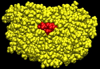
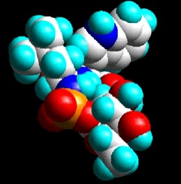
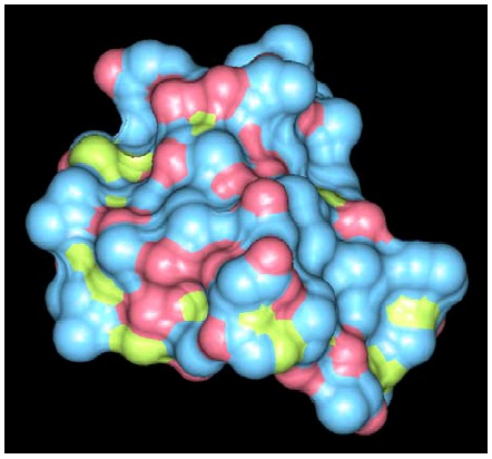
Figure 35. HIV-1 Protease
A space filling representation of HIV-1 protease (yellow) with an inhibitory drug (red) blocking its binding site.
This representation allows for visualization, but it brings us no closer to being able to
computationally decide which parts of which atoms are on the surface of the protein and which are
buried inside the structure. Some additional tool is needed to capture notions of interior and
exterior and spatial adjacency.
Representing Shape
Using the sphere model for atoms, one way to define the shape of a molecule is as the union of
(possibly overlapping) balls in R 3 .
Figure 36. Space Filling Diagram
The space filling diagram models each atom as a sphere in 3D.
Since proteins inside our cells are in an aqueous environment, considering a protein's interactions
with solvent molecules, particularly water, is very important for appropriately modeling them.
Recall that one of the phenomena that determines the structure of a protein is the hydrophobic
effect: some amino acid residues are stabilized by the presence of water, and others are repelled.
The extent of the interaction of a protein with the surrounding water depends on the surface area
of the protein that can be reached by water molecules. Therefore, quantitave modeling of the
strength of interaction with solvent often involves computing the solvent accessible surface area
(SASA). Computing SASA can be done by regarding each solvent molecule as a sphere of set
radius. This is of course a simplification, since water molecules are not spherical. When this
sphere rolls about the molecule, its center delineates the SASA. One can think of the SASA of a
molecule as the result of growing each atom sphere by the radius of the solvent sphere. Instead, by
taking what is swept out by the front of the solvent sphere, we obtain the molecular surface (MS)
model of the molecule. Alternatively, the MS can be obtained by removing a layer of solvent
radius depth from the SASA model.
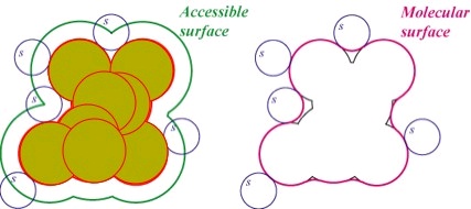
<db:title> VDW
Representation
<db:title> Accessible Surface Area </db:title>
</db:title>
(a) Each atom can be modeled as a (b) Not all molecular surface is accessible to solvent due to the existence of small cavities.
Van der Waals sphere in three
Rolling a solvent ball over the Van der Waals spheres traces out the surface area experienced by
dimensions. The union of the
the solvent. Solvent accessible surface area (SASA) is a very important measure for
spheres gives the molecular
quantitatively determining the behavior and interaction tendencies of a protein.
surface.
Figure 37. Representations of Molecular Shape
Two different notions and representations of the surface of a molecule.
The surface determined by SASA analysis depends on the size of a typical solvent molecule. The
larger the solvent, the less contoured the resulting surface will appear, because a larger probe
molecules would not be able to fit into some of the interatomic spaces that a smaller one would.
<db:title> Probing the surface area with a
<db:title> Probing the surface area with a
solvent ball of radius 1.5 Å</db:title>
solvent ball of radius 1.4 Å</db:title>
(a) Typically, solvent is modeled as a ball of radius 1.4 Å. This
(b) Increasing the radius of the solvent ball reduces the solvent
delineates the solvent accessible surface shown.
accessible surface area because there are more cavities that a
bulkier ball cannot penetrate.
Figure 38. Solvent Accessible Surface Area
Solvent-accessible surface area (SASA) for two different solvent radii.
Alpha-Shapes
Part of the problem with defining the shape of a protein is that we start with nothing but a point
set, and the "shape" of a set of discontinuous points is poorly defined. The problem is, what do we
mean by shape? As you saw above, the shape of a molecule depends on what is being used to
measure it. To handle this ambiguity, we will introduce a method of shape calculation based on a
parameter, α, which will determine the radius of a spherical probe that will define the surface. The
method defines a class of shapes, called α-shapes [link] for any given point set. It allows fast, accurate, and efficient calculations of volume and surface area.
α-shapes are a generalization of the convex hull. Consider a point set S. Define an α-ball as a
sphere of radius α. An α-ball is empty if it contains no points in S. For any α between zero and
infinity, the α-hull of S is the complement of the union of all empty α-balls.
For α of infinity, the α-shape is the convex hull of S.
For α smaller than the 1/2 smallest distance between two points in S, the α-shape is S itself.
For any α in between, one can think of the α-hull as the largest polygon (polyhedron) or set
thereof whose vertices are in the point set and whose edges are of length less than 2α. The
presence of an edge indicates that a probe of radius α cannot pass between the edge endpoints.
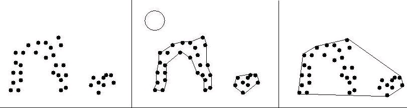
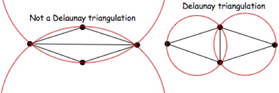
Figure 39. Two-Dimensional α-Shapes
Some α-shapes are shown for a point set and various values of α. On the left, α is 0 or slightly more, such that an α-ball can fit between any two points in the set. The α-shape is therefore the original point set. On the right, α is infinity, so an α-ball can be approximated locally by a line. α on this scale yields the convex hull of the point set. The middle image shows the α-shape for α equal to the radius of the ball shown. This yields two disjoint boundaries, one of which has a significant indentation. Voids, or empty pockets completely enclosed by the α-shape, are also possible, for instance if the α-shape is ring-like (in 2D) or forms a hollow shell (in 3D).
Computing the Alpha-Shape: Delaunay Triangulation
A triangulation of a three-dimensional point set S is any decomposition of S into non-
intersecting tetrahedra (triangles for two-dimensional point sets). The Delaunay triangulation of
S is the unique triangulation of S satisfying the additional requirement that no sphere
circumscribing a tetrahedron in the triangulation contains any point in S. Although it is incidental
to α-shapes, it is worth noting that the Delaunay triangulation maximizes the average of the
smallest angle over all triangles. In other words, it favors relatively even-sided triangles over
sharp and stretched ones.
Figure 40. Two-Dimensional Delaunay Triangulation
The Delaunay triangulation of the four points given is shown on the right. Note that the circumscribing circles on the left each contain one point of S, whereas the circles on the right do not. The transition from the triangulation on the left to that on the right is called an edge flip, and is the basic operation of constructing a two-dimensional Delaunay triangulation. Face flipping is the analogous procedure for five points in three dimensions.
The Delaunay triangulation of a point set is usually calculated by an incremental flip algorithm as
follows:
The points of S are sorted on one coordinate (x, y, or z). This step is not strictly necessary but
makes the algorithm run faster than if the points were in arbitrary order.
Each point is added in sorted order. Upon adding a point:

The point is connected to previously added points that are "visible" to it, that is, to points to
which it can be connected by a line segment without passing through a face of a tetrahedron.
Any new tetrhedra formed are checked and flipped if necessary.
Any tetrahedra adjacent to flipped tetrahedra are checked and flipped. This continues until
further flipping is unnecessary, which is guaranteed to occur
This algorithm runs in worst case O(n^2) time, but expected O(n^(3/2)) time. Without the
sort in the first step, the expected case would be O(n log n). A full description and analysis of
Delaunay triangulation algorithms is given in [1] [link], chapter 9.
From the Delaunay triangulation the α-shape is computed by removing all edges, triangles, and
tetrahedra that have circumscribing spheres with radius greater than α. Formally, the α-complex
is the part of the Delaunay triangulation that remains after removing edges longer than α. The α-
shape is the boundary of the α-complex.
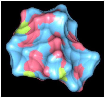
Pockets [link] can be detected by comparing the α-shape to the whole Delauney triangulation.
Missing tetrahedra represent indentations, concavity, and generally negative space in the overall
volume occupied by the protein. Particularly large or deep pockets may indicate a substrate
binding site.
Weighted Alpha Shapes
Regular α-shapes can be extended to deal with varying weights (i.e., spheres with different radii,
such as different types of atoms) [link]. The formal definitions become complicated, but the key idea is to use a pseudo distance measure that uses the weights. Suppose we have two atoms at
positions p1 and p2 with weights w1 and w2. Then the pseudo distance is defined as the square of
the Euclidean distance minus the weights. The pseudo distance is zero if and only if two spheres
centered at p1 and p2 with radii equal to sqrt(w1) and sqrt(w2) are just touching.
Figure 41.
Pseudo distance to account for atoms of different sizes.
Calculating Molecular Volume Using α-Shapes
The volume of a molecule can be approximated using the space-filling model, in which each atom
is modeled as a ball whose radius is α, where α is selected depending on the model being used:
Van der Waals surface, molecular surface, solvent accessible surface, etc. Unfortunately,
calculating the volume is not as simple as taking the sum of the ball volumes because they may
overlap. Calculating the volume of a complex of overlapping balls is non-trivial because of the
overlaps. If two spheres overlap, the volume is the sum of the volumes of the spheres minus the
volume of the overlap, which was counted twice. If three overlap, the volume is the sum of the
ball volumes, minus the volume of each pairwise overlap, plus the volume of the three-way
overlap, which was subtracted one too many times in accounting for the pairwise overlaps. In the
general case, all pairwise, three-way, four-way and so on to n-way intersections (assuming there
are n atoms) must be considered. Proteins generally have thousands or tens of thousands of atoms,
so the general n-way case may be computationally expensive and may introduce numerical error.
Figure 42.
Three overlapping discs (balls if three dimensional). Calculating the total area (volume if three dimensional) of the balls requires summing the areas of each ball, then subtracting out the pairwise intersection areas, since each was counted once for each ball it is inside. Then the intersection area of the three balls must be added back because, although it was added three times initially, it was also subtracted once in each of the three pairwise intersections. In the general case, with n balls, all of which may overlap, intersections of odd numbers of balls are added, and intersections of even numbers of balls subtracted, to calculate the total area or volume.
α-shapes provide a way around this undesirable combinatorial complexity [link], and this issue has been one of the motivating factors for introducing α-shapes. To calculate the volume of a
protein, we take the sum of all ball volumes, then subtract only those pairwise intersections for
which a corresponding edge exists in the α-complex. Only those three-way intersections for which
the corresponding triangle is in the α-complex must then be added back. Finally, only four-way
intersections corresponding to tetrahedra in the α-complex need to be subtracted. No higher-order
intersections are necessary, and the number of volume calculations necessary corresponds directly
to the complexity of the α-complex, which is O(n log n) in the number of atoms.
An example of how this approach works is given on page 4 of the Liang et al. article in the Recommended Reading section below. A proof of correctness and derivation is also provided in
the article. Surface area calculations, such as solvent-accessible surface area, which is often used
to estimate the strength of interactions between a protein and the solvent molecules surrounding
it, are made by a similar use of the α-complex.
Recommended Reading
H. Edelsbrunner, D. Kirkpatrick, and R. Seidel. [PDF]. "On the Shape of a Set of Points in the Plane." IEEE Transactions on Information Theory, 29(4):551-559, 1983. This is the original α-
shapes paper (caution: the definition of α is different from that used in later papers--it is the
negative reciprocal of α as presented above).
H. Edelsbrunner and E.P. Mucke. [PDF]. "Three-dimensional Alpha Shapes." Workshop on Volume Visualization, Boston, MA. pp 75-82. 1992. This article shows how to extend α-shapes
to three-dimensional point sets.
J. Liang, H. Edelsbrunner, P. Fu, P.V. Sudhakar, and S. Subramaniam. [PDF] . Analytical shape computation of macromolecules: I. molecular area and volume through alpha shape. Proteins:
Structure, Function, and Genetics, 33:1-17, 1998. This is a paper on using α-shapes to speed up
volume and surface area calculations for molecular models.
H. Edelsbrunner, M.Facello and Jie Liang. [PDF] . On the definition and the construction of pockets in macromolecules. Discrete and Applied Mathematics, 88:83-102, 1998.
Software
An α-shapes applet. This applet lets you display α-shapes, Voronoi diagrams, and Delauney triangulations for arbitrary point sets and variable α (use the slider at the bottom). Be cautioned
that this applet uses the original definition of α, which is -1/α as we defined α above for three-
dimensional point sets.
A small example showing how α-shapes can be used to identify pockets.
Computational geometry software (CGAL), which includes demo programs for alpha shapes, Delaunay triangulations, etc.
Locating binding sites in protein structures (including use of α-shapes).
References
1. de Berg, M. and van Krefeld, M. and Overmars, M. and Schwarzkopf, O. (2000).
Computational Geometry: Algorithms and Applications. (Second). Springer.
2. J. Liang and H. Edelsbrunner and P. Fu and P.V. Sudhakar and S. Subramaniam. (1998).
Analytical shape computation of macromolecules: I. molecular area and volume through alpha
shape. [http://www3.interscience.wiley.com/cgi-bin/abstract/36315/ABSTRACT]. Proteins:
Structure, Function, and Genetics, 33, 1-17.
3. H. Edelsbrunner and M.Facello and Jie Liang. (1998). On the definition and the construction of
pockets in macromolecules. [http://dx.doi.org/10.1016/S0166-218X(98)00067-5]. Discrete and
Applied Mathematics, 88, 83-102.
4. H. Edelsbrunner and E. P. Mücke. (1994). Three-Dimensional Alpha-Shapes.
[http://portal.acm.org/citation.cfm?id=156635]. ACM Transaction on Graphics, 13, 43-72.
5. E. W. Weisstein. (2005). Circle-Circle Intersection. [http://mathworld.wolfram.com/Circle-
CircleIntersection.html]. MathWorld.
6. E. W. Weisstein. (2005). Sphere-Sphere Intersection. [http://mathworld.wolfram.com/Sphere-
SphereIntersection.html]. MathWorld.
7. E. W. Weisstein. (2005). Cayley-Menger Determinant.
[http://mathworld.wolfram.com/Cayley-MengerDeterminant.html]. MathWorld.
Molecular Distance Measures
Topics in this Module
Comparing Molecular Conformations
Optimal Alignment for lRMSD Using Rotation Matrices
Optimal Alignment for lRMSD Using Quaternions
Quaternions and Three-Dimensional Rotations
Optimal Alignment with Quaternions
Intramolecular Distance and Related Measures
Comparing Molecular Conformations
Molecules are not rigid. On the contrary, they are highly flexible objects, capable of changing
shape dramatically through the rotation of dihedral angles. We need a measure to express how
much a molecule changes going from one conformation to another, or alternatively, how different
two conformations are from each other. Each distinct shape of a given molecule is called a
conformation. Although one could conceivably compute the volume of the intersection of the
alpha shapes for two conformations (see Molecular Shapes and Surfaces for an explanation of alpha shapes) to measure the shape change, this is prohibitively computationally expensive.
Simpler measures of distance between conformations have been defined, based on variables such
as the Cartesian coordinates for each atom, or the bond and torsion angles within the molecule.
When working with Cartesian coordinates, one can represent a molecular conformation as a vector
whose components are the Cartesian coordinates of the molecule's atoms. Therefore, a
conformation for a molecule with N atoms can be represented as a 3N-dimensional vector of real
numbers.
RMSD and lRMSD
One of the most widely accepted difference measures for conformations of a molecule is least
root mean square deviation (lRMSD). To calculate the RMSD of a pair of structures (say x and
y), each structure must be represented as a 3N-length (assuming N atoms) vector of coordinates.
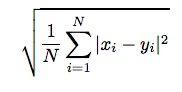
The RMSD is the square root of the average of the squared distances between corresponding
atoms of x and y. It is a measure of the average atomic displacement between the two
conformations:
However, when molecular conformations are sampled from molecular dynamics or other forms of
sampling, it is often the case that the molecule drifts away from the origin and rotates in an
arbitrary way. The lRMSD distance aims at compensating for these facts by representing the
minimum RMSD over all possible relative positions and orientations of the two conformations
under consideration. Calculating the lRMSD consists of first finding an optimal alignment of the
two structures, and then calculating their RMSD. Note that aligning two conformations may
require both a translation and rotat