Geometric Methods in Structural Computational Biology by Lydia Kavraki - HTML preview
Download the book in PDF, ePub, Kindle for a complete version.

Geometric Methods in Structural Computational
Biology
By: Lydia Kavraki
Online: < http://cnx.org/content/col10344/1.6>
This selection and arrangement of content as a collection is copyrighted by Lydia Kavraki.
It is licensed under the Creative Commons Attribution License: http://creativecommons.org/licenses/by/2.0/
Collection structure revised: 2007/06/11
For copyright and attribution information for the modules contained in this collection, see the " Attributions" section at the end of the collection.
Geometric Methods in Structural Computational
Biology
Table of Contents
Structural Computational Biology: Introduction and Background
Proteins and Their Significance to Biology and Medicine
Experimental Methods for Protein Structure Determination
Structure Prediction of Large Complexes
Protein Structure Repositories
Visualizing Protein Structures
Visualizing HLA-AW with Protein Explorer
Representing Proteins in Silico and Protein Forward Kinematics
Modeling Proteins on a Computer
Cartesian Representation of Protein Conformations
The Internal Degrees of Freedom of a Protein
Dihedral Representation of Protein Conformations
Mathematical Background: Matrices and Transformations
Denavit-Hartenberg Local Frames
Protein Inverse Kinematics and the Loop Closure Problem
Inverse Kinematics and its Relevance to Proteins
Classic Inverse Kinematics Methods
Inverse Kinematics Methods with Optimization
Cyclic Coordinate Descent and Its Application to Proteins
Computing the Alpha-Shape: Delaunay Triangulation
Calculating Molecular Volume Using α-Shapes
Comparing Molecular Conformations
Optimal Alignment for lRMSD Using Rotation Matrices
Optimal Alignment for lRMSD Using Quaternions
Quaternions and Three-Dimensional Rotations
Optimal Alignment with Quaternions
Intramolecular Distance and Related Measures
Protein Classification, Local Alignment, and Motifs
Local Matching: Geometric Hashing, Pose Clustering and Match Augmentation
Dimensionality Reduction Methods for Molecular Motion
Isometric Feature Mapping (Isomap)
Robotic Path Planning and Protein Modeling
Proteins as Robotic Manipulators
Sampling Based Planners for Proteins
Motion Planning for Proteins: Biophysics and Applications
Free Energy and Potential Functions
Van der Waals Interactions and Steric Clash
An Example: The CHARMM All-Atom Empirical Potential
Applications of Roadmap Methods
Stochastic Roadmap Simulations
Protein-Ligand Docking Pathways and Kinetics
Protein-Ligand Docking, Including Flexible Receptor-Flexible Ligand Docking
Components of a Docking Program
Explicit force field scoring function
Knowledge-based scoring functions
Parameterization of the Problem
Examples of rigid-receptor docking programs
Selection of Specific Degrees of Freedom
Chapter 1. Homework assignments
1.1. Assignment 1: Visualization and Ranking of Protein Conformations
Visualizing Protein Conformations
A. Visualizing a Set of Conformations
Visualizing Protein Substructures
Structurally Classifying Proteins
1.2. Assignment 2: Performing Rotations
"Defining the Connnectivity of a Backbone Chain"
1.3. Assignment 3: Inverse Kinematics
Motivation for Inverse Kinematics in Proteins
Inverse Kinematics for a Polypeptide Chain
Structural Computational Biology: Introduction and
Background
Topics in this Module
Proteins and Their Significance to Biology and Medicine
Experimental Methods for Protein Structure Determination
Protein Structure Repositories
Visualizing Protein Structures
Proteins and Their Significance to Biology and Medicine
Proteins are the molecular workhorses of all known biological systems. Among other functions,
they are the motors that cause muscle contraction, the catalysts that drive life-sustaining chemical
processes, and the molecules that hold cells together to form tissues and organs.
The following is a list of a few of the diverse biological processes mediated by proteins:
Proteins called enzymes catalyse vital reactions, such as those involved in metabolism, cellular
reproduction, and gene expression.
Regulatory proteins control the location and timing of gene expression.
Cytokines, hormones, and other signalling proteins transmit information between cells.
Immune system proteins recognize and tag foreign material for attack and removal.
Structural proteins prevent cells from collapsing on themselves, as well as forming large
structures such as hair, nails, and the protective, largely impermeable outer layer of skin. They
also provide a framework along which molecules can be transported within cells.
The estimate of the number of genes in the human genome has been changing dramatically since it
was annotated (the latest gene count estimates can be found in this Wikipedia article on the
human genome). Each gene encodes one or more distinct proteins. The total number of distinct proteins in the human body is larger than the number of genes due to alternate splicing. Of those, only a small fraction have been isolated and studied to the point that their purpose and mechanism
of activity is well understood. If the functions and relationships between every protein were fully
understood, we would most likely have a much better understanding of how our bodies work and
what goes wrong in diseases such as cancer, amyotrophic lateral sclerosis, Parkinson's, heart
disease and many others. As a result, protein science is a very active field. As the field has
progressed, computer-aided modeling and simulation of proteins have found their place among the
methods available to researchers.
Protein Structure
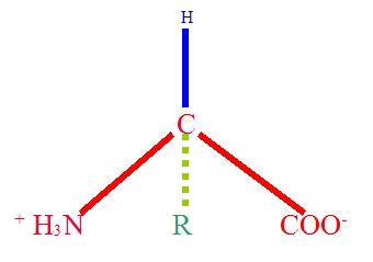
An amino acid is a simple organic molecule consisting of a basic (hydrogen-accepting), amine
group bound to an acidic (hydrogen-donating) carboxyl group via a single intermediate carbon
atom:
Figure 1. An α-amino acid
A generic α-amino acid. The "R" group is variable, and is the only difference between the 20 common amino acids. This form is called a zwitterion, because it has both positive and negatively charged atoms. The zwitterionic state results from the amine group (NH2) gaining a hydrogen atom from solution, and the acidic group (COO) losing one.
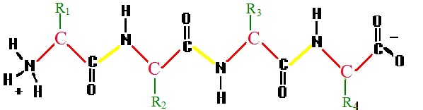
During the translation of a gene into a protein, the protein is formed by the sequential joining of
amino acids end-to-end to form a long chain-like molecule, or polymer. A polymer of amino
acids is often referred to as a polypeptide. The genome is capable of coding for 20 different
amino acids whose chemical properties depend on the composition of their side chains ("R" in the
above figure). Thus, to a first approximation, a protein is nothing more than a sequence of these
amino acids (or, more properly, amino acid residues, because both the amine and acid groups lose
their acid/base properties when they are part of a polypeptide). This sequence is called the
primary structure of the protein.
Figure 2. A polypeptide
A generic polypeptide chain. The bonds shown in yellow, which connect separate amino acid residues, are called peptide bonds.


The Wikipedia entry on amino acids provides a more detailed background, including the structure, properties, abbreviations, and genetic codes for each of the 20 common amino acids.
The primary structure of a protein is easily obtainable from its corresponding gene sequence, as
well as by experimental manipulation. Unfortunately, the primary structure is only indirectly
related to the protein's function. In order to work properly, a protein must fold to form a specific
three-dimensional shape, called its native structure or native conformation. The three-
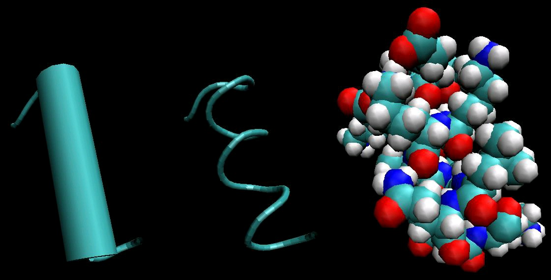
dimensional structure of a protein is usually understood in a hierarchical manner. Secondary
structure refers to folding in a small part of the protein that forms a characteristic shape. The
most common secondary structure elements are α-helices and β-sheets, one or both of which are
present in almost all natural proteins.
Figure 3. Secondary Structure: α-helix
α-helices, rendered three different ways. Left is a typical cartoon rendering, in which the helix is depicted as a cylinder. Center shows a trace of the backbone of the protein. Right shows a space-filling model of the helix, and is the only rendering that shows all atoms (including those on side chains).
<db:title> Bond representation
<db:title> Cartoon
</db:title>
<db:title> Ribbon
representation </db:title>
representation </db:title>
(c) Each segment in this representation
represents a bond. Unlike the other two
(a) Different parts of the polypeptide
(b) β-sheets are sometimes referred to as β
representations, side chains are illustrated.
strand align with each other to form a β- pleated sheets, because of the regular zig- Note the alignment of oxygen atoms (red) sheet. This β-sheet is anti-parallel,
zag of the strands evident in this
toward nitrogen atoms (blue) on adjacent
because adjacent segments of the protein representation.
strands. This alignment is due to hydrogen
run in opposite directions.
bonding, the primary interaction involved in
stabilizing secondary structure.
Figure 4. Secondary Structure: β-sheet
Beta-sheets represented in three different rendering modes: cartoon, ribbon, and bond representations.
Tertiary structure refers to structural elements formed by bringing more distant parts of a chain
together into structural domains. The spatial arrangement of these domains with respect to each
other is also considered part of the tertiary structure. Finally, many proteins consist of more than
one polypeptide folded together, and the spatial relationship between these separate polypeptide
chains is called the quaternary structure. It is important to note that the native conformation of a
protein is a direct consequence of its primary sequence and its chemical environment, which for
most proteins is either aqueous solution with a biological pH (roughly neutral) or the oily interior
of a cell membrane. Nevertheless, no reliable computational method exists to predict the native
structure from the amino acid sequence, and this is a topic of ongoing research. Thus, in order to
find the native structure of a protein, experimental techniques are deployed. The most common
approaches are outlined in the next section.
Experimental Methods for Protein Structure Determination
A structure of a protein is a three-dimensional arrangement of the atoms such that the integrity of
the molecule (its connectivity) is maintained. The goal of a protein structure determination
experiment is to find a set of three-dimensional (x, y, z) coordinates for each atom of the molecule
in some natural state. Of particular interest is the native structure, that is, the structure assumed by
the protein under its biological conditions, as well as structures assumed by the protein when in
the process of interacting with other molecules. Brief sketches of the major structure
determination methods follow:
X-ray Crystallography
The most commonly used and usually highest-resolution method of structure determination is x-
ray crystallography. To obtain structures by this method, laboratory biochemists obtain a very
pure, crystalline sample of a protein. X-rays are then passed through the sample, in which they are
diffracted by the electrons of each atom of the protein. The diffraction pattern is recorded, and can
be used to reconstruct the three-dimensional pattern of electron density, and therefore, within
some error, the location of each atom. A high-resolution crystal structure has a resolution on the
order of 1 to 2 Angstroms (Å). One Angstrom is the diameter of a hydrogen atom (10^-10 meter,
or one hundred-millionth of a centimeter).
Unlike other structure determination methods, with x-ray crystallography, there is no fundamental
limit on the size of the molecule or complex to be studied. However, in order for the method to
work, a pure, crystalline sample of the protein must be obtained. For many proteins, including
many membrane-bound receptors, this is not possible. In addition, a single x-ray diffraction
experiment provides only static information - that is, it provides only information about the native
structure of the protein under the particular experimental conditions used. As we will see later,
proteins are often flexible, dynamic objects when in their natural state in solution, so a single
structure, while useful, may not tell the full story. More information on X-ray Crystallography is
available at Crystallography 101 and in the Wikipedia.
NMR
Nuclear Magnetic Resonance (NMR) spectroscopy has recently come into its own as a protein
structure determination method. In an NMR experiment, a very strong magnetic field is
transiently applied to a sample of the protein being studied, forcing any magnetic atomic nuclei
into alignment. The signal given off by a nucleus as it returns to an unaligned state is
characteristic of its chemical environment. Information about the atoms within two chemical
bonds of the resonating nucleus can be deduced, and, more importantly, information about which
atoms are spatially near each other can also be found. The latter information leads to a large
system of distance constraints between the atoms of the protein, which can then be solved to find a
three-dimensional structure. Resolution of NMR structures is variable and depends strongly on the
flexibility of the protein. Because NMR is performed on proteins in solution, they are free to
undergo spatial rearrangements, so for flexible parts of the protein, there may be many more than
one detectable structures. In fact, NMR structures are generally reported as ensembles of 20-50
distinct structures. This makes NMR the only structure determination technique suited to
elucidating the behavior of intrinsically unstructured proteins, that is, proteins that lack a well-
defined tertiary structure. The reported ensemble may also provide insight into the dynamics of
the protein, that is, the ways in which it tends to move.
NMR structure determination is generally limited to proteins smaller than 25-30 kilodaltons
(kDa), because the signals from different atoms start to overlap and become difficult to resolve in
that range. Additionally, the proteins must be soluble in concentrations of 0.2-0.5 mM without
aggregation or precipitation. For more information on how NMR is used to find molecular