who, among many other contributions to quantum mechanics, formulated a mathematical treatment of the wave nature of matter that used matrices
rather than wave equations. We will deal with some specifics in later sections, but it is worth noting that de Broglie’s work was a watershed for the
development of quantum mechanics. De Broglie was awarded the Nobel Prize in 1929 for his vision, as were Davisson and G. P. Thomson in 1937
for their experimental verification of de Broglie’s hypothesis.
Figure 29.22 This diffraction pattern was obtained for electrons diffracted by crystalline silicon. Bright regions are those of constructive interference, while dark regions are those of destructive interference. (credit: Ndthe, Wikimedia Commons)
CHAPTER 29 | INTRODUCTION TO QUANTUM PHYSICS 1049
Example 29.7 Electron Wavelength versus Velocity and Energy
For an electron having a de Broglie wavelength of 0.167 nm (appropriate for interacting with crystal lattice structures that are about this size): (a)
Calculate the electron’s velocity, assuming it is nonrelativistic. (b) Calculate the electron’s kinetic energy in eV.
Strategy
For part (a), since the de Broglie wavelength is given, the electron’s velocity can be obtained from λ = h / p by using the nonrelativistic formula
for momentum, p = mv. For part (b), once v is obtained (and it has been verified that v is nonrelativistic), the classical kinetic energy is
simply (1 / 2) mv 2 .
Solution for (a)
Substituting the nonrelativistic formula for momentum ( p = mv ) into the de Broglie wavelength gives
(29.36)
λ = hp = hmv.
Solving for v gives
(29.37)
v = h
mλ.
Substituting known values yields
(29.38)
v =
6.63×10⁻³⁴ J ⋅ s
= 4.36×10⁶ m/s.
(9.11×10⁻³¹ kg)(0.167×10⁻⁹ m)
Solution for (b)
While fast compared with a car, this electron’s speed is not highly relativistic, and so we can comfortably use the classical formula to find the
electron’s kinetic energy and convert it to eV as requested.
(29.39)
KE = 12 mv 2
= 12(9.11×10⁻³¹ kg)(4.36×10⁶ m/s)2
= (86.4×10⁻¹⁸ J)⎛
1 eV
⎞
⎝1.602×10⁻¹⁹ J⎠
= 54.0 eV
Discussion
This low energy means that these 0.167-nm electrons could be obtained by accelerating them through a 54.0-V electrostatic potential, an easy
task. The results also confirm the assumption that the electrons are nonrelativistic, since their velocity is just over 1% of the speed of light and
the kinetic energy is about 0.01% of the rest energy of an electron (0.511 MeV). If the electrons had turned out to be relativistic, we would have
had to use more involved calculations employing relativistic formulas.
Electron Microscopes
One consequence or use of the wave nature of matter is found in the electron microscope. As we have discussed, there is a limit to the detail
observed with any probe having a wavelength. Resolution, or observable detail, is limited to about one wavelength. Since a potential of only 54 V can
produce electrons with sub-nanometer wavelengths, it is easy to get electrons with much smaller wavelengths than those of visible light (hundreds of
nanometers). Electron microscopes can, thus, be constructed to detect much smaller details than optical microscopes. (See Figure 29.23.)
There are basically two types of electron microscopes. The transmission electron microscope (TEM) accelerates electrons that are emitted from a hot
filament (the cathode). The beam is broadened and then passes through the sample. A magnetic lens focuses the beam image onto a fluorescent
screen, a photographic plate, or (most probably) a CCD (light sensitive camera), from which it is transferred to a computer. The TEM is similar to the
optical microscope, but it requires a thin sample examined in a vacuum. However it can resolve details as small as 0.1 nm ( 10−10 m ), providing
magnifications of 100 million times the size of the original object. The TEM has allowed us to see individual atoms and structure of cell nuclei.
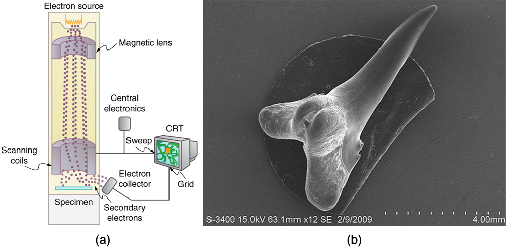
The scanning electron microscope (SEM) provides images by using secondary electrons produced by the primary beam interacting with the surface
of the sample (see Figure 29.23). The SEM also uses magnetic lenses to focus the beam onto the sample. However, it moves the beam around
electrically to “scan” the sample in the x and y directions. A CCD detector is used to process the data for each electron position, producing images
like the one at the beginning of this chapter. The SEM has the advantage of not requiring a thin sample and of providing a 3-D view. However, its
resolution is about ten times less than a TEM.
1050 CHAPTER 29 | INTRODUCTION TO QUANTUM PHYSICS
Figure 29.23 Schematic of a scanning electron microscope (SEM) (a) used to observe small details, such as those seen in this image of a tooth of a Himipristis, a type of shark (b). (credit: Dallas Krentzel, Flickr)
Electrons were the first particles with mass to be directly confirmed to have the wavelength proposed by de Broglie. Subsequently, protons, helium
nuclei, neutrons, and many others have been observed to exhibit interference when they interact with objects having sizes similar to their de Broglie
wavelength. The de Broglie wavelength for massless particles was well established in the 1920s for photons, and it has since been observed that all
massless particles have a de Broglie wavelength λ = h / p. The wave nature of all particles is a universal characteristic of nature. We shall see in
following sections that implications of the de Broglie wavelength include the quantization of energy in atoms and molecules, and an alteration of our
basic view of nature on the microscopic scale. The next section, for example, shows that there are limits to the precision with which we may make
predictions, regardless of how hard we try. There are even limits to the precision with which we may measure an object’s location or energy.
Making Connections: A Submicroscopic Diffraction Grating
The wave nature of matter allows it to exhibit all the characteristics of other, more familiar, waves. Diffraction gratings, for example, produce
diffraction patterns for light that depend on grating spacing and the wavelength of the light. This effect, as with most wave phenomena, is most
pronounced when the wave interacts with objects having a size similar to its wavelength. For gratings, this is the spacing between multiple slits.)
When electrons interact with a system having a spacing similar to the electron wavelength, they show the same types of interference patterns as
light does for diffraction gratings, as shown at top left in Figure 29.24.
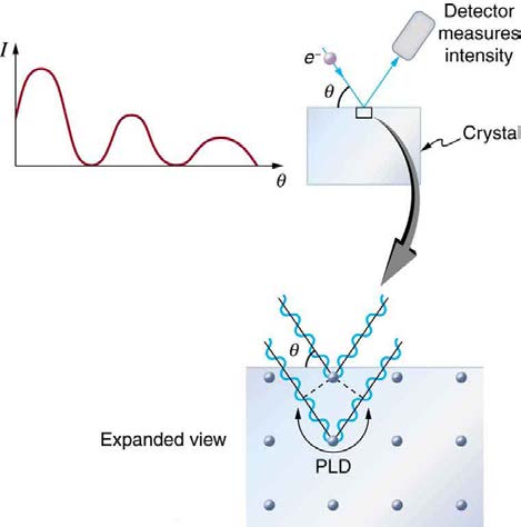
Atoms are spaced at regular intervals in a crystal as parallel planes, as shown in the bottom part of Figure 29.24. The spacings between these
planes act like the openings in a diffraction grating. At certain incident angles, the paths of electrons scattering from successive planes differ by
one wavelength and, thus, interfere constructively. At other angles, the path length differences are not an integral wavelength, and there is partial
to total destructive interference. This type of scattering from a large crystal with well-defined lattice planes can produce dramatic interference
patterns. It is called Bragg reflection, for the father-and-son team who first explored and analyzed it in some detail. The expanded view also
shows the path-length differences and indicates how these depend on incident angle θ in a manner similar to the diffraction patterns for x rays
reflecting from a crystal.
Figure 29.24 The diffraction pattern at top left is produced by scattering electrons from a crystal and is graphed as a function of incident angle relative to the regular array of atoms in a crystal, as shown at bottom. Electrons scattering from the second layer of atoms travel farther than those scattered from the top layer. If the path length
difference (PLD) is an integral wavelength, there is constructive interference.
CHAPTER 29 | INTRODUCTION TO QUANTUM PHYSICS 1051
Let us take the spacing between parallel planes of atoms in the crystal to be d . As mentioned, if the path length difference (PLD) for the
electrons is a whole number of wavelengths, there will be constructive interference—that is, PLD = nλ( n = 1, 2, 3, … ) . Because
AB = BC = d sin θ, we have constructive interference when nλ = 2 d sin θ. This relationship is called the Bragg equation and applies not
only to electrons but also to x rays.
The wavelength of matter is a submicroscopic characteristic that explains a macroscopic phenomenon such as Bragg reflection. Similarly, the
wavelength of light is a submicroscopic characteristic that explains the macroscopic phenomenon of diffraction patterns.
29.7 Probability: The Heisenberg Uncertainty Principle
Probability Distribution
Matter and photons are waves, implying they are spread out over some distance. What is the position of a particle, such as an electron? Is it at the
center of the wave? The answer lies in how you measure the position of an electron. Experiments show that you will find the electron at some definite
location, unlike a wave. But if you set up exactly the same situation and measure it again, you will find the electron in a different location, often far
outside any experimental uncertainty in your measurement. Repeated measurements will display a statistical distribution of locations that appears
wavelike. (See Figure 29.25.)
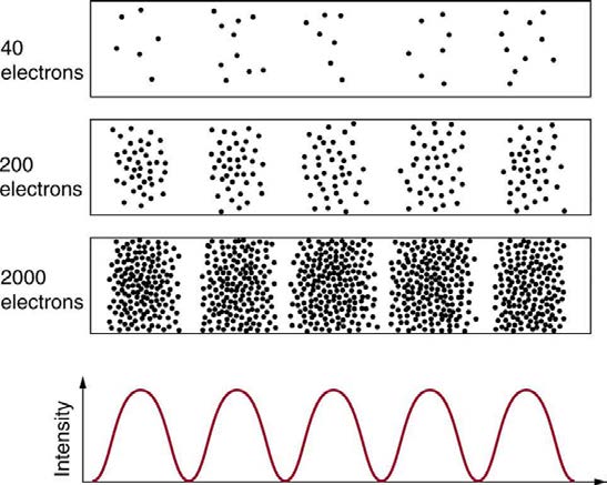
Figure 29.25 The building up of the diffraction pattern of electrons scattered from a crystal surface. Each electron arrives at a definite location, which cannot be precisely
predicted. The overall distribution shown at the bottom can be predicted as the diffraction of waves having the de Broglie wavelength of the electrons.
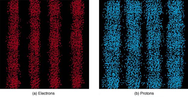
Figure 29.26 Double-slit interference for electrons (a) and photons (b) is identical for equal wavelengths and equal slit separations. Both patterns are probability distributions in the sense that they are built up by individual particles traversing the apparatus, the paths of which are not individually predictable.
After de Broglie proposed the wave nature of matter, many physicists, including Schrödinger and Heisenberg, explored the consequences. The idea
quickly emerged that, because of its wave character, a particle’s trajectory and destination cannot be precisely predicted for each particle individually.
However, each particle goes to a definite place (as illustrated in Figure 29.25). After compiling enough data, you get a distribution related to the
particle’s wavelength and diffraction pattern. There is a certain probability of finding the particle at a given location, and the overall pattern is called a
probability distribution. Those who developed quantum mechanics devised equations that predicted the probability distribution in various
circumstances.
It is somewhat disquieting to think that you cannot predict exactly where an individual particle will go, or even follow it to its destination. Let us explore
what happens if we try to follow a particle. Consider the double-slit patterns obtained for electrons and photons in Figure 29.26. First, we note that
these patterns are identical, following d sin θ = mλ , the equation for double-slit constructive interference developed in Photon Energies and the
Electromagnetic Spectrum, where d is the slit separation and λ is the electron or photon wavelength.

1052 CHAPTER 29 | INTRODUCTION TO QUANTUM PHYSICS
Both patterns build up statistically as individual particles fall on the detector. This can be observed for photons or electrons—for now, let us
concentrate on electrons. You might imagine that the electrons are interfering with one another as any waves do. To test this, you can lower the
intensity until there is never more than one electron between the slits and the screen. The same interference pattern builds up! This implies that a
particle’s probability distribution spans both slits, and the particles actually interfere with themselves. Does this also mean that the electron goes
through both slits? An electron is a basic unit of matter that is not divisible. But it is a fair question, and so we should look to see if the electron
traverses one slit or the other, or both. One possibility is to have coils around the slits that detect charges moving through them. What is observed is
that an electron always goes through one slit or the other; it does not split to go through both. But there is a catch. If you determine that the electron
went through one of the slits, you no longer get a double slit pattern—instead, you get single slit interference. There is no escape by using another
method of determining which slit the electron went through. Knowing the particle went through one slit forces a single-slit pattern. If you do not
observe which slit the electron goes through, you obtain a double-slit pattern.
Heisenberg Uncertainty
How does knowing which slit the electron passed through change the pattern? The answer is fundamentally important— measurement affects the
system being observed. Information can be lost, and in some cases it is impossible to measure two physical quantities simultaneously to exact
precision. For example, you can measure the position of a moving electron by scattering light or other electrons from it. Those probes have
momentum themselves, and by scattering from the electron, they change its momentum in a manner that loses information. There is a limit to
absolute knowledge, even in principle.
Figure 29.27 Werner Heisenberg was one of the best of those physicists who developed early quantum mechanics. Not only did his work enable a description of nature on the
very small scale, it also changed our view of the availability of knowledge. Although he is universally recognized for his brilliance and the importance of his work (he received
the Nobel Prize in 1932, for example), Heisenberg remained in Germany during World War II and headed the German effort to build a nuclear bomb, permanently alienating
himself from most of the scientific community. (credit: Author Unknown, via Wikimedia Commons)
It was Werner Heisenberg who first stated this limit to knowledge in 1929 as a result of his work on quantum mechanics and the wave characteristics
of all particles. (See Figure 29.27). Specifically, consider simultaneously measuring the position and momentum of an electron (it could be any
particle). There is an uncertainty in position Δ x that is approximately equal to the wavelength of the particle. That is,
(29.40)
Δ x ≈ λ.
As discussed above, a wave is not located at one point in space. If the electron’s position is measured repeatedly, a spread in locations will be
observed, implying an uncertainty in position Δ x . To detect the position of the particle, we must interact with it, such as having it collide with a
detector. In the collision, the particle will lose momentum. This change in momentum could be anywhere from close to zero to the total momentum of
the particle, p = h / λ . It is not possible to tell how much momentum will be transferred to a detector, and so there is an uncertainty in momentum
Δ p , too. In fact, the uncertainty in momentum may be as large as the momentum itself, which in equation form means that
(29.41)
Δ p ≈ hλ.
The uncertainty in position can be reduced by using a shorter-wavelength electron, since Δ x ≈ λ . But shortening the wavelength increases the
uncertainty in momentum, since Δ p ≈ h / λ . Conversely, the uncertainty in momentum can be reduced by using a longer-wavelength electron, but
this increases the uncertainty in position. Mathematically, you can express this trade-off by multiplying the uncertainties. The wavelength cancels,
leaving
(29.42)
Δ xΔ p ≈ h.
So if one uncertainty is reduced, the other must increase so that their product is ≈ h .
With the use of advanced mathematics, Heisenberg showed that the best that can be done in a simultaneous measurement of position and
momentum is
CHAPTER 29 | INTRODUCTION TO QUANTUM PHYSICS 1053
(29.43)
Δ xΔ p ≥ h
4π.
This is known as the Heisenberg uncertainty principle. It is impossible to measure position x and momentum p simultaneously with uncertainties
Δ x and Δ p that multiply to be less than h / 4π . Neither uncertainty can be zero. Neither uncertainty can become small without the other becoming
large. A small wavelength allows accurate position measurement, but it increases the momentum of the probe to the point that it further disturbs the
momentum of a system being measured. For example, if an electron is scattered from an atom and has a wavelength small enough to detect the
position of electrons in the atom, its momentum can knock the electrons from their orbits in a manner that loses information about their original
motion. It is therefore impossible to follow an electron in its orbit around an atom. If you measure the electron’s position, you will find it in a definite
location, but the atom will be disrupted. Repeated measurements on identical atoms will produce interesting probability distributions for electrons
around the atom, but they will not produce motion information. The probability distributions are referred to as electron clouds or orbitals. The shapes
of these orbitals are often shown in general chemistry texts and are discussed in The Wave Nature of Matter Causes Quantization.
Example 29.8 Heisenberg Uncertainty Principle in Position and Momentum for an Atom
(a) If the position of an electron in an atom is measured to an accuracy of 0.0100 nm, what is the electron’s uncertainty in velocity? (b) If the
electron has this velocity, what is its kinetic energy in eV?
Strategy
The uncertainty in position is the accuracy of the measurement, or Δ x = 0.0100 nm . Thus the smallest uncertainty in momentum Δ p can be
calculated using Δ xΔ p ≥ h/4 π . Once the uncertainty in momentum Δ p is found, the uncertainty in velocity can be found from Δ p = mΔ v .
Solution for (a)
Using the equals sign in the uncertainty principle to express the minimum uncertainty, we have
(29.44)
Δ xΔ p = h
4π.
Solving for Δ p and substituting known values gives
(29.45)
Δ p = h
4πΔ x = 6.63×10⁻³⁴ J ⋅ s = 5.28×10⁻²⁴ kg ⋅ m/s.
4π(1.00×10⁻¹¹ m)
Thus,
(29.46)
Δ p = 5.28×10⁻²⁴ kg ⋅ m/s = mΔ v.
Solving for Δ v and substituting the mass of an electron gives
(29.47)
Δ v = Δ p
m = 5.28×10⁻²⁴ kg ⋅ m/s = 5.79×10⁶ m/s.
9.11×10⁻³¹ kg
Solution for (b)
Although large, this velocity is not highly relativistic, and so the electron’s kinetic energy is
(29.48)
KE e = 12 mv 2
= 12(9.11×10⁻³¹ kg)(5.79×10⁶ m/s)2
= (1.53×10⁻¹⁷ J)⎛
1 eV
⎞
⎝1.60×10⁻¹⁹ J⎠ = 95.5 eV.
Discussion
Since atoms are roughly 0.1 nm in size, knowing the position of an electron to 0.0100 nm localizes it reasonably well inside the atom. This would
be like being able to see details one-tenth the size of the atom. But the consequent uncertainty in velocity is large. You certainly could not follow
it very well if its velocity is so uncertain. To get a further idea of how large the uncertainty in velocity is, we assumed the velocity of the electron
was equal to its uncertainty and found this gave a kinetic energy of 95.5 eV. This is significantly greater than the typical energy difference
between levels in atoms (see Table 29.1), so that it is impossible to get a meaningful energy for the electron if we know its position even
moderately well.
Why don’t we notice Heisenberg’s uncertainty principle in everyday life? The answer is that Planck’s constant is very small. Thus the lower limit in the
uncertainty of measuring the position and momentum of large objects is negligible. We can detect sunlight reflected from Jupiter and follow the planet
in its orbit around the Sun. The reflected sunlight alters the momentum of Jupiter and creates an uncertainty in its momentum, but this is totally
negligible compared with Jupiter’s huge momentum. The correspondence principle tells us that the predictions of quantum mechanics become
indistinguishable from classical physics for large objects, which is the case here.
Heisenberg Uncertainty for Energy and Time
There is another form of Heisenberg’s uncertainty principle for simultaneous measurements of energy and time. In equation form,
1054 CHAPTER 29 | INTRODUCTION TO QUANTUM PHYSICS
(29.49)
Δ EΔ t ≥ h
4π,
where Δ E is the uncertainty in energy and Δ t is the uncertainty in time. This means that within a time interval Δ t , it is not possible to measure energy precisely—there will be an uncertainty Δ E in the measurement. In order to measure energy more precisely (to make Δ E smaller), we must
increase Δ t . This time interval may be the amount of time we take to make the measurement, or it could be the amount of time a particular state
exists, as in the next Example 29.9.
Example 29.9 Heisenberg Uncertainty Principle for Energy and Time for an Atom
An atom in an excited state temporarily stores energy. If the lifetime of this excited state is measured to be 1.0×10⁻¹⁰ s , what is the minimum
uncertainty in the energy of the state in eV?
Strategy
The minimum uncertainty in energy Δ E is found by using the equals sign in Δ EΔ t ≥ h/4 π and corresponds to a reasonable choice for the
uncertainty in time. The largest the uncertainty in time can be is the full lifetime of the excited state, or Δ t = 1.0×10⁻¹⁰ s .
Solution
Solving the uncertainty principle for Δ E and substituting known values gives
(29.50)
Δ E = h
4πΔt = 6.63×10⁻³⁴ J ⋅ s = 5.3×10⁻²⁵ J.
4π(1.0×10⁻¹⁰ s)
Now converting to eV yields
(29.51)
Δ E = (5.3×10⁻²⁵ J)⎛
1 eV
⎞
⎝1.6×10⁻¹⁹ J⎠ = 3.3×10⁻⁶ eV.
Discussion
The lifetime of 10−10 s is typical of excited states in atoms—on human time scales, they quickly emit their stored energy. An uncertainty in
energy of only a few millionths of a
Describe what you're looking for in as much detail as you'd like.
Our AI reads your request and finds the best matching books for you.
Popular searches:
Join 2.9 million readers and get unlimited free ebooks