College Physics (2012) by Manjula Sharma, Paul Peter Urone, et al - HTML preview
Download the book in PDF, ePub, Kindle for a complete version.
22.6 The Hall Effect
We have seen effects of a magnetic field on free-moving charges. The magnetic field also affects charges moving in a conductor. One result is the
Hall effect, which has important implications and applications.
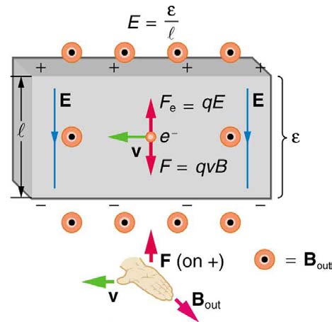
Figure 22.27 shows what happens to charges moving through a conductor in a magnetic field. The field is perpendicular to the electron drift velocity and to the width of the conductor. Note that conventional current is to the right in both parts of the figure. In part (a), electrons carry the current and
move to the left. In part (b), positive charges carry the current and move to the right. Moving electrons feel a magnetic force toward one side of the
conductor, leaving a net positive charge on the other side. This separation of charge creates a voltage ε , known as the Hall emf, across the
conductor. The creation of a voltage across a current-carrying conductor by a magnetic field is known as the Hall effect, after Edwin Hall, the
American physicist who discovered it in 1879.
Figure 22.27 The Hall effect. (a) Electrons move to the left in this flat conductor (conventional current to the right). The magnetic field is directly out of the page, represented by circled dots; it exerts a force on the moving charges, causing a voltage ε , the Hall emf, across the conductor. (b) Positive charges moving to the right (conventional current also to the right) are moved to the side, producing a Hall emf of the opposite sign, –ε . Thus, if the direction of the field and current are known, the sign of the charge carriers
can be determined from the Hall effect.
One very important use of the Hall effect is to determine whether positive or negative charges carries the current. Note that in Figure 22.27(b), where
positive charges carry the current, the Hall emf has the sign opposite to when negative charges carry the current. Historically, the Hall effect was
used to show that electrons carry current in metals and it also shows that positive charges carry current in some semiconductors. The Hall effect is
used today as a research tool to probe the movement of charges, their drift velocities and densities, and so on, in materials. In 1980, it was
discovered that the Hall effect is quantized, an example of quantum behavior in a macroscopic object.
The Hall effect has other uses that range from the determination of blood flow rate to precision measurement of magnetic field strength. To examine
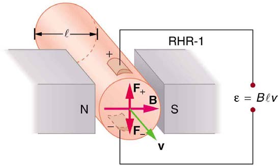
these quantitatively, we need an expression for the Hall emf, ε , across a conductor. Consider the balance of forces on a moving charge in a situation
where B , v , and l are mutually perpendicular, such as shown in Figure 22.28. Although the magnetic force moves negative charges to one side, they cannot build up without limit. The electric field caused by their separation opposes the magnetic force, F = qvB , and the electric force,
F e = qE , eventually grows to equal it. That is,
qE
(22.10)
= qvB
or
E
(22.11)
= vB.
Note that the electric field E is uniform across the conductor because the magnetic field B is uniform, as is the conductor. For a uniform electric
field, the relationship between electric field and voltage is E = ε / l , where l is the width of the conductor and ε is the Hall emf. Entering this into the last expression gives
ε
(22.12)
l = vB.
Solving this for the Hall emf yields
ε
(22.13)
= Blv ( B, v, and l, mutually perpendicular) ,
where ε is the Hall effect voltage across a conductor of width l through which charges move at a speed v .
788 CHAPTER 22 | MAGNETISM
Figure 22.28 The Hall emf ε produces an electric force that balances the magnetic force on the moving charges. The magnetic force produces charge separation, which
builds up until it is balanced by the electric force, an equilibrium that is quickly reached.
One of the most common uses of the Hall effect is in the measurement of magnetic field strength B . Such devices, called Hall probes, can be made
very small, allowing fine position mapping. Hall probes can also be made very accurate, usually accomplished by careful calibration. Another
application of the Hall effect is to measure fluid flow in any fluid that has free charges (most do). (See Figure 22.29.) A magnetic field applied
perpendicular to the flow direction produces a Hall emf ε as shown. Note that the sign of ε depends not on the sign of the charges, but only on the
directions of B and v . The magnitude of the Hall emf is ε = Blv , where l is the pipe diameter, so that the average velocity v can be determined from ε providing the other factors are known.
Figure 22.29 The Hall effect can be used to measure fluid flow in any fluid having free charges, such as blood. The Hall emf ε is measured across the tube perpendicular to the applied magnetic field and is proportional to the average velocity v .
Example 22.3 Calculating the Hall emf: Hall Effect for Blood Flow
A Hall effect flow probe is placed on an artery, applying a 0.100-T magnetic field across it, in a setup similar to that in Figure 22.29. What is the Hall emf, given the vessel’s inside diameter is 4.00 mm and the average blood velocity is 20.0 cm/s?
Strategy
Because B , v , and l are mutually perpendicular, the equation ε = Blv can be used to find ε .
Solution
Entering the given values for B , v , and l gives
(22.14)
ε = Blv = (0.100 T)⎛⎝4.00×10⁻³ m⎞⎠(0.200 m/s)
= 80.0 μV
Discussion
This is the average voltage output. Instantaneous voltage varies with pulsating blood flow. The voltage is small in this type of measurement. ε is
particularly difficult to measure, because there are voltages associated with heart action (ECG voltages) that are on the order of millivolts. In
CHAPTER 22 | MAGNETISM 789
practice, this difficulty is overcome by applying an AC magnetic field, so that the Hall emf is AC with the same frequency. An amplifier can be
very selective in picking out only the appropriate frequency, eliminating signals and noise at other frequencies.
22.7 Magnetic Force on a Current-Carrying Conductor
Because charges ordinarily cannot escape a conductor, the magnetic force on charges moving in a conductor is transmitted to the conductor itself.
Figure 22.30 The magnetic field exerts a force on a current-carrying wire in a direction given by the right hand rule 1 (the same direction as that on the individual moving
charges). This force can easily be large enough to move the wire, since typical currents consist of very large numbers of moving charges.
We can derive an expression for the magnetic force on a current by taking a sum of the magnetic forces on individual charges. (The forces add
because they are in the same direction.) The force on an individual charge moving at the drift velocity v d is given by F = qv d B sin θ . Taking B to be uniform over a length of wire l and zero elsewhere, the total magnetic force on the wire is then F = ( qv d B sin θ)( N) , where N is the number of charge carriers in the section of wire of length l . Now, N = nV , where n is the number of charge carriers per unit volume and V is the volume of wire in the field. Noting that V = Al , where A is the cross-sectional area of the wire, then the force on the wire is F = ( qv d B sin θ)( nAl) .
Gathering terms,
F
(22.15)
= ( nqAv d) lB sin θ.
Because nqAv d = I (see Current),
F
(22.16)
= IlB sin θ
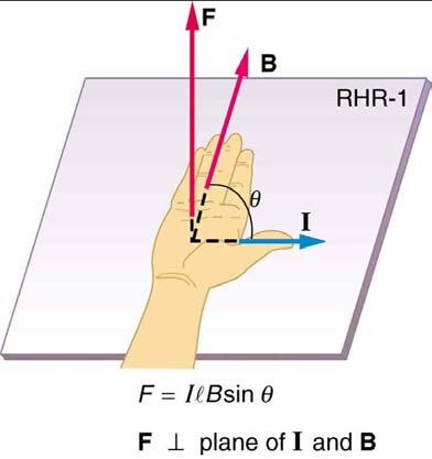
is the equation for magnetic force on a length l of wire carrying a current I in a uniform magnetic field B , as shown in Figure 22.31. If we divide
both sides of this expression by l , we find that the magnetic force per unit length of wire in a uniform field is Fl = IB sin θ . The direction of this force is given by RHR-1, with the thumb in the direction of the current I . Then, with the fingers in the direction of B , a perpendicular to the palm
points in the direction of F , as in Figure 22.31.
Figure 22.31 The force on a current-carrying wire in a magnetic field is F = IlB sin θ . Its direction is given by RHR-1.
790 CHAPTER 22 | MAGNETISM
Example 22.4 Calculating Magnetic Force on a Current-Carrying Wire: A Strong Magnetic Field
Calculate the force on the wire shown in Figure 22.30, given B = 1.50 T , l = 5.00 cm , and I = 20.0 A .
Strategy
The force can be found with the given information by using F = IlB sin θ and noting that the angle θ between I and B is 90º , so that sin θ = 1 .
Solution
Entering the given values into F = IlB sin θ yields
F
(22.17)
= IlB sin θ = (20.0 A)(0.0500 m)(1.50 T)(1).
The units for tesla are 1 T =
N
A ⋅ m ; thus,
F
(22.18)
= 1.50 N.
Discussion
This large magnetic field creates a significant force on a small length of wire.
Magnetic force on current-carrying conductors is used to convert electric energy to work. (Motors are a prime example—they employ loops of wire
and are considered in the next section.) Magnetohydrodynamics (MHD) is the technical name given to a clever application where magnetic force
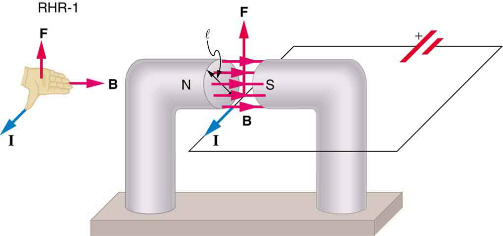
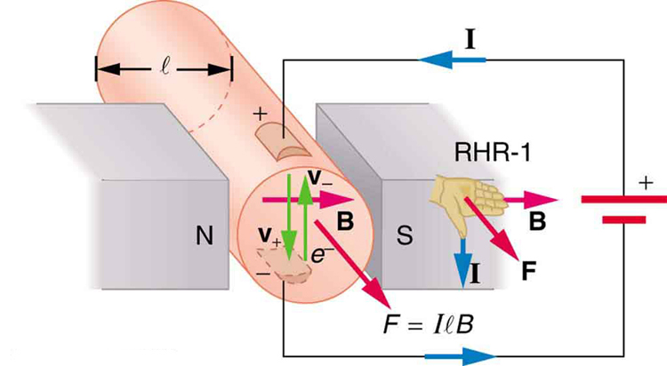
pumps fluids without moving mechanical parts. (See Figure 22.32.)
Figure 22.32 Magnetohydrodynamics. The magnetic force on the current passed through this fluid can be used as a nonmechanical pump.
A strong magnetic field is applied across a tube and a current is passed through the fluid at right angles to the field, resulting in a force on the fluid
parallel to the tube axis as shown. The absence of moving parts makes this attractive for moving a hot, chemically active substance, such as the
liquid sodium employed in some nuclear reactors. Experimental artificial hearts are testing with this technique for pumping blood, perhaps
circumventing the adverse effects of mechanical pumps. (Cell membranes, however, are affected by the large fields needed in MHD, delaying its
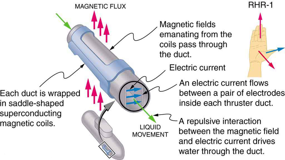
practical application in humans.) MHD propulsion for nuclear submarines has been proposed, because it could be considerably quieter than
conventional propeller drives. The deterrent value of nuclear submarines is based on their ability to hide and survive a first or second nuclear strike.
As we slowly disassemble our nuclear weapons arsenals, the submarine branch will be the last to be decommissioned because of this ability (See
Figure 22.33.) Existing MHD drives are heavy and inefficient—much development work is needed.
Figure 22.33 An MHD propulsion system in a nuclear submarine could produce significantly less turbulence than propellers and allow it to run more silently. The development
of a silent drive submarine was dramatized in the book and the film The Hunt for Red October.
CHAPTER 22 | MAGNETISM 791
22.8 Torque on a Current Loop: Motors and Meters
Motors are the most common application of magnetic force on current-carrying wires. Motors have loops of wire in a magnetic field. When current is
passed through the loops, the magnetic field exerts torque on the loops, which rotates a shaft. Electrical energy is converted to mechanical work in
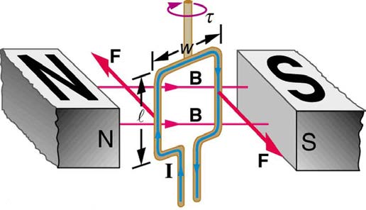
the process. (See Figure 22.34.)
Figure 22.34 Torque on a current loop. A current-carrying loop of wire attached to a vertically rotating shaft feels magnetic forces that produce a clockwise torque as viewed
from above.
Let us examine the force on each segment of the loop in Figure 22.34 to find the torques produced about the axis of the vertical shaft. (This will lead to a useful equation for the torque on the loop.) We take the magnetic field to be uniform over the rectangular loop, which has width w and height l .
First, we note that the forces on the top and bottom segments are vertical and, therefore, parallel to the shaft, producing no torque. Those vertical
forces are equal in magnitude and opposite in direction, so that they also produce no net force on the loop. Figure 22.35 shows views of the loop
from above. Torque is defined as τ = rF sin θ , where F is the force, r is the distance from the pivot that the force is applied, and θ is the angle between r and F . As seen in Figure 22.35(a), right hand rule 1 gives the forces on the sides to be equal in magnitude and opposite in direction, so that the net force is again zero. However, each force produces a clockwise torque. Since r = w / 2 , the torque on each vertical segment is
( w / 2) F sin θ , and the two add to give a total torque.
(22.19)
τ = w 2 F sin θ + w 2 F sin θ = wF sin θ
792 CHAPTER 22 | MAGNETISM
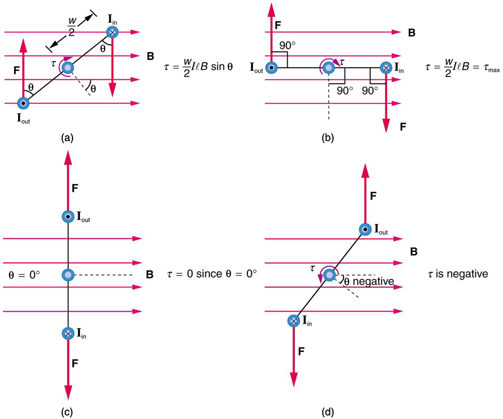
Figure 22.35 Top views of a current-carrying loop in a magnetic field. (a) The equation for torque is derived using this view. Note that the perpendicular to the loop makes an
angle θ with the field that is the same as the angle between w / 2 and F . (b) The maximum torque occurs when θ is a right angle and sin θ = 1 . (c) Zero (minimum) torque occurs when θ is zero and sin θ = 0 . (d) The torque reverses once the loop rotates past θ = 0 .
Now, each vertical segment has a length l that is perpendicular to B , so that the force on each is F = IlB . Entering F into the expression for torque yields
τ
(22.20)
= wIlB sin θ.
If we have a multiple loop of N turns, we get N times the torque of one loop. Finally, note that the area of the loop is A = wl ; the expression for
the torque becomes
τ
(22.21)
= NIAB sin θ.
This is the torque on a current-carrying loop in a uniform magnetic field. This equation can be shown to be valid for a loop of any shape. The loop
carries a current I , has N turns, each of area A , and the perpendicular to the loop makes an angle θ with the field B . The net force on the loop is zero.
Example 22.5 Calculating Torque on a Current-Carrying Loop in a Strong Magnetic Field
Find the maximum torque on a 100-turn square loop of a wire of 10.0 cm on a side that carries 15.0 A of current in a 2.00-T field.
Strategy
Torque on the loop can be found using τ = NIAB sin θ . Maximum torque occurs when θ = 90º and sin θ = 1 .
Solution
For sin θ = 1 , the maximum torque is
τ
(22.22)
max = NIAB.
Entering known values yields
(22.23)
τ max = (100)(15.0 A)⎛⎝0.100 m2⎞⎠(2.00 T)
= 30.0 N ⋅ m.
CHAPTER 22 | MAGNETISM 793
Discussion
This torque is large enough to be useful in a motor.
The torque found in the preceding example is the maximum. As the coil rotates, the torque decreases to zero at θ = 0 . The torque then reverses its
direction once the coil rotates past θ = 0 . (See Figure 22.35(d).) This means that, unless we do something, the coil will oscillate back and forth about equilibrium at θ = 0 . To get the coil to continue rotating in the same direction, we can reverse the current as it passes through θ = 0 with
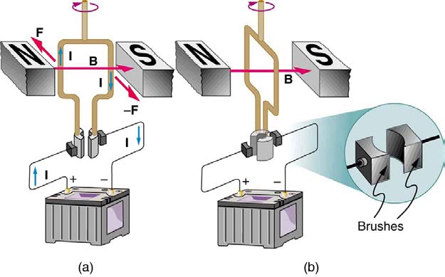
automatic switches called brushes. (See Figure 22.36.)
Figure 22.36 (a) As the angular momentum of the coil carries it through θ = 0 , the brushes reverse the current to keep the torque clockwise. (b) The coil will rotate
continuously in the clockwise direction, with the current reversing each half revolution to maintain the clockwise torque.
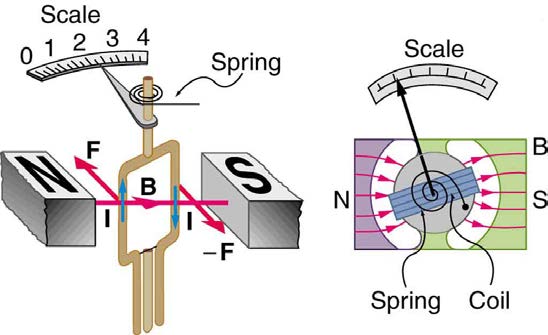
Meters, such as those in analog fuel gauges on a car, are another common application of magnetic torque on a current-carrying loop. Figure 22.37
shows that a meter is very similar in construction to a motor. The meter in the figure has its magnets shaped to limit the effect of θ by making B
perpendicular to the loop over a large angular range. Thus the torque is proportional to I and not θ . A linear spring exerts a counter-torque that
balances the current-produced torque. This makes the needle deflection proportional to I . If an exact proportionality cannot be achieved, the gauge
reading can be calibrated. To produce a galvanometer for use in analog voltmeters and ammeters that have a low resistance and respond to small
currents, we use a large loop area A , high magnetic field B , and low-resistance coils.
Figure 22.37 Meters are very similar to motors but only rotate through a part of a revolution. The magnetic poles of this meter are shaped to keep the component of B
perpendicular to the loop constant, so that the torque does not depend on θ and the deflection against the return spring is proportional only to the current I .
22.9 Magnetic Fields Produced by Currents: Ampere’s Law
How much current is needed to produce a significant magnetic field, perhaps as strong as the Earth’s field? Surveyors will tell you that overhead
electric power lines create magnetic fields that interfere with their compass readings. Indeed, when Oersted discovered in 1820 that a current in a
wire affected a compass needle, he was not dealing with extremely large currents. How does the shape of wires carrying current affect the shape of
the magnetic field created? We noted earlier that a current loop created a magnetic field similar to that of a bar magnet, but what about a straight wire
or a toroid (doughnut)? How is the direction of a current-created field related to the direction of the current? Answers to these questions are explored
in this section, together with a brief discussion of the law governing the fields created by currents.
794 CHAPTER 22 | MAGNETISM
Magnetic Field Created by a Long Straight Current-Carrying Wire: Right Hand Rule 2
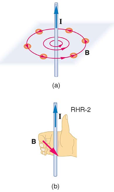
Magnetic fields have both direction and magnitude. As noted before, one way to explore the direction of a magnetic field is with compasses, as
shown for a long straight current-carrying wire in Figure 22.38. Hall probes can determine the magnitude of the field. The field around a long straight wire is found to be in circular loops. The right hand rule 2 (RHR-2) emerges from this exploration and is valid for any current segment— point the
thumb in the direction of the current, and the fingers curl in the direction of the magnetic field loops created by it.
Figure 22.38 (a) Compasses placed near a long straight current-carrying wire indicate that field lines form circular loops centered on the wire. (b) Right hand rule 2 states that, if the right hand thumb points in the direction of the current, the fingers curl in the direction of the field. This rule is consistent with the field mapped for the long straight wire and is valid for any current segment.
The magnetic field strength (magnitude) produced by a long straight current-carrying wire is found by experiment to be
(22.24)
B = µ 0 I
2 πr (long straight wire) ,
where I is the current, r is the shortest distance to the wire, and the constant µ 0 = 4π × 10−7 T ⋅ m/A is the permeability of free space. ( µ 0
is one of the basic constants in nature. We will see later that µ 0 is related to the speed of light.) Since the wire is very long, the magnitude of the
field depends only on distance from the wire r , not on position along the wire.
Example 22.6 Calculating Current that Produces a Magnetic Field
Find the current in a long straight wire that would produce a magnetic field twice the strength of the Earth’s at a distance of 5.0 cm from the wire.
Strategy
The Earth’s field is about 5.0×10⁻⁵ T , and so here B due to the wire is taken to be 1.0×10⁻⁴ T . The equation B = µ 0 I
2 πr can be used to
find I , since all other quantities are known.
Solution
Solving for I and entering known values gives
⎛
(22.25)