College Physics (2012) by Manjula Sharma, Paul Peter Urone, et al - HTML preview
Download the book in PDF, ePub, Kindle for a complete version.
1018 m distance light travels in a century
peta
P
1015
petasecond Ps
1015 s
30 million years
tera
T
1012
terawatt
TW
1012 W powerful laser output
giga
G
109
gigahertz
GHz 109 Hz
a microwave frequency
mega
M
106
megacurie MCi 106 Ci
high radioactivity
kilo
k
103
kilometer
km
103 m
about 6/10 mile
hecto
h
102
hectoliter
hL
102 L
26 gallons
deka
da
101
dekagram
dag
101 g
teaspoon of butter
—
—
100 (=1)
deci
d
10−1
deciliter
dL
10−1 L less than half a soda
centi
c
10−2
centimeter cm
10−2 m fingertip thickness
milli
m
10−3
millimeter
mm
10−3 m flea at its shoulders
micro
µ
10−6
micrometer µm
10−6 m detail in microscope
nano
n
10−9
nanogram
ng
10−9 g small speck of dust
pico
p
10−12
picofarad
pF
10−12 F small capacitor in radio
femto
f
10−15
femtometer fm
10−15 m size of a proton
atto
a
10−18
attosecond as
10−18 s time light crosses an atom
Known Ranges of Length, Mass, and Time
The vastness of the universe and the breadth over which physics applies are illustrated by the wide range of examples of known lengths, masses,
and times in Table 1.3. Examination of this table will give you some feeling for the range of possible topics and numerical values. (See Figure 1.20
and Figure 1.21.)
Figure 1.20 Tiny phytoplankton swims among crystals of ice in the Antarctic Sea. They range from a few micrometers to as much as 2 millimeters in length. (credit: Prof.
Gordon T. Taylor, Stony Brook University; NOAA Corps Collections)
1. See Appendix A for a discussion of powers of 10.
22 CHAPTER 1 | INTRODUCTION: THE NATURE OF SCIENCE AND PHYSICS
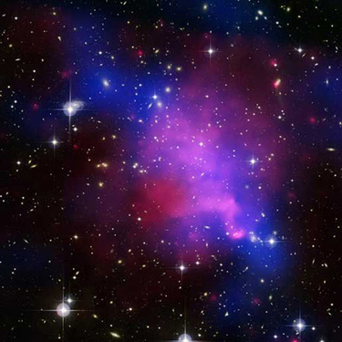
Figure 1.21 Galaxies collide 2.4 billion light years away from Earth. The tremendous range of observable phenomena in nature challenges the imagination. (credit: NASA/
CXC/UVic./A. Mahdavi et al. Optical/lensing: CFHT/UVic./H. Hoekstra et al.)
Unit Conversion and Dimensional Analysis
It is often necessary to convert from one type of unit to another. For example, if you are reading a European cookbook, some quantities may be
expressed in units of liters and you need to convert them to cups. Or, perhaps you are reading walking directions from one location to another and
you are interested in how many miles you will be walking. In this case, you will need to convert units of feet to miles.
Let us consider a simple example of how to convert units. Let us say that we want to convert 80 meters (m) to kilometers (km).
The first thing to do is to list the units that you have and the units that you want to convert to. In this case, we have units in meters and we want to
convert to kilometers.
Next, we need to determine a conversion factor relating meters to kilometers. A conversion factor is a ratio expressing how many of one unit are
equal to another unit. For example, there are 12 inches in 1 foot, 100 centimeters in 1 meter, 60 seconds in 1 minute, and so on. In this case, we
know that there are 1,000 meters in 1 kilometer.
Now we can set up our unit conversion. We will write the units that we have and then multiply them by the conversion factor so that the units cancel
out, as shown:
(1.1)
80m× 1 km
1000m = 0.080 km.
Note that the unwanted m unit cancels, leaving only the desired km unit. You can use this method to convert between any types of unit.
Click Section C.1 for a more complete list of conversion factors.
CHAPTER 1 | INTRODUCTION: THE NATURE OF SCIENCE AND PHYSICS 23
Table 1.3 Approximate Values of Length, Mass, and Time
Masses in kilograms (more precise
Times in seconds (more precise
Lengths in meters
values in parentheses)
values in parentheses)
Mass of an electron
10−18 Present experimental limit to smallest
⎛
observable detail
10−30
10−23 Time for light to cross a proton
⎝9.11×10⁻³¹ kg⎞⎠
Mass of a hydrogen atom
10−15 Diameter of a proton
10−27 ⎛
10−22 Mean life of an extremely unstable
⎝1.67×10⁻²⁷ kg⎞⎠
nucleus
10−14 Diameter of a uranium nucleus
10−15 Mass of a bacterium
10−15 Time for one oscillation of visible
light
10−10 Diameter of a hydrogen atom
10−5 Mass of a mosquito
10−13 Time for one vibration of an atom
in a solid
10−8 Thickness of membranes in cells of living
organisms
10−2 Mass of a hummingbird
10−8 Time for one oscillation of an FM
radio wave
10−6 Wavelength of visible light
1
Mass of a liter of water (about a
quart)
10−3 Duration of a nerve impulse
10−3 Size of a grain of sand
102
Mass of a person
1
Time for one heartbeat
1
Height of a 4-year-old child
103
Mass of a car
105
One day ⎛⎝8.64×10⁴ s⎞⎠
102
Length of a football field
108
Mass of a large ship
107
One year (y) ⎛⎝3.16×10⁷ s⎞⎠
104
Greatest ocean depth
1012 Mass of a large iceberg
109
About half the life expectancy of a
human
107
Diameter of the Earth
1015 Mass of the nucleus of a comet
1011 Recorded history
1011 Distance from the Earth to the Sun
1023 Mass of the Moon ⎛⎝7.35×10²² kg⎞⎠ 1017 Age of the Earth
1016 Distance traveled by light in 1 year (a light
year)
1025 Mass of the Earth ⎛⎝5.97×1024 kg⎞⎠ 1018 Age of the universe
1021 Diameter of the Milky Way galaxy
1030 Mass of the Sun ⎛⎝1.99×1030 kg⎞⎠
1022 Distance from the Earth to the nearest large
galaxy (Andromeda)
1042 Mass of the Milky Way galaxy
(current upper limit)
1026 Distance from the Earth to the edges of the
known universe
1053 Mass of the known universe (current
upper limit)
Example 1.1 Unit Conversions: A Short Drive Home
Suppose that you drive the 10.0 km from your university to home in 20.0 min. Calculate your average speed (a) in kilometers per hour (km/h) and
(b) in meters per second (m/s). (Note: Average speed is distance traveled divided by time of travel.)
Strategy
First we calculate the average speed using the given units. Then we can get the average speed into the desired units by picking the correct
conversion factor and multiplying by it. The correct conversion factor is the one that cancels the unwanted unit and leaves the desired unit in its
place.
Solution for (a)
(1) Calculate average speed. Average speed is distance traveled divided by time of travel. (Take this definition as a given for now—average
speed and other motion concepts will be covered in a later module.) In equation form,
(1.2)
average speed =distance
time .
(2) Substitute the given values for distance and time.
(1.3)
average speed = 10.0 km
20.0 min = 0.500 km
min.
(3) Convert km/min to km/h: multiply by the conversion factor that will cancel minutes and leave hours. That conversion factor is 60 min/hr .
Thus,
(1.4)
average speed =0.500 km
min×60 min
1 h = 30.0 km
h .
24 CHAPTER 1 | INTRODUCTION: THE NATURE OF SCIENCE AND PHYSICS
Discussion for (a)
To check your answer, consider the following:
(1) Be sure that you have properly cancelled the units in the unit conversion. If you have written the unit conversion factor upside down, the units
will not cancel properly in the equation. If you accidentally get the ratio upside down, then the units will not cancel; rather, they will give you the
wrong units as follows:
(1.5)
km
km ⋅ hr
min× 1 hr
60 min = 1
60 min2 ,
which are obviously not the desired units of km/h.
(2) Check that the units of the final answer are the desired units. The problem asked us to solve for average speed in units of km/h and we have
indeed obtained these units.
(3) Check the significant figures. Because each of the values given in the problem has three significant figures, the answer should also have
three significant figures. The answer 30.0 km/hr does indeed have three significant figures, so this is appropriate. Note that the significant figures
in the conversion factor are not relevant because an hour is defined to be 60 minutes, so the precision of the conversion factor is perfect.
(4) Next, check whether the answer is reasonable. Let us consider some information from the problem—if you travel 10 km in a third of an hour
(20 min), you would travel three times that far in an hour. The answer does seem reasonable.
Solution for (b)
There are several ways to convert the average speed into meters per second.
(1) Start with the answer to (a) and convert km/h to m/s. Two conversion factors are needed—one to convert hours to seconds, and another to
convert kilometers to meters.
(2) Multiplying by these yields
(1.6)
Average speed = 30.0km
h × 1 h
3,600 s×1,000 m
1 km ,
(1.7)
Average speed = 8.33ms.
Discussion for (b)
If we had started with 0.500 km/min, we would have needed different conversion factors, but the answer would have been the same: 8.33 m/s.
You may have noted that the answers in the worked example just covered were given to three digits. Why? When do you need to be concerned
about the number of digits in something you calculate? Why not write down all the digits your calculator produces? The module Accuracy,
Precision, and Significant Figures will help you answer these questions.
Nonstandard Units
While there are numerous types of units that we are all familiar with, there are others that are much more obscure. For example, a firkin is a unit
of volume that was once used to measure beer. One firkin equals about 34 liters. To learn more about nonstandard units, use a dictionary or
encyclopedia to research different “weights and measures.” Take note of any unusual units, such as a barleycorn, that are not listed in the text.
Think about how the unit is defined and state its relationship to SI units.
Some hummingbirds beat their wings more than 50 times per second. A scientist is measuring the time it takes for a hummingbird to beat its
wings once. Which fundamental unit should the scientist use to describe the measurement? Which factor of 10 is the scientist likely to use to
describe the motion precisely? Identify the metric prefix that corresponds to this factor of 10.
Solution
The scientist will measure the time between each movement using the fundamental unit of seconds. Because the wings beat so fast, the scientist
will probably need to measure in milliseconds, or 10−3 seconds. (50 beats per second corresponds to 20 milliseconds per beat.)
One cubic centimeter is equal to one milliliter. What does this tell you about the different units in the SI metric system?
Solution
The fundamental unit of length (meter) is probably used to create the derived unit of volume (liter). The measure of a milliliter is dependent on the
measure of a centimeter.
CHAPTER 1 | INTRODUCTION: THE NATURE OF SCIENCE AND PHYSICS 25
1.3 Accuracy, Precision, and Significant Figures
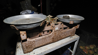
Figure 1.22 A double-pan mechanical balance is used to compare different masses. Usually an object with unknown mass is placed in one pan and objects of known mass are
placed in the other pan. When the bar that connects the two pans is horizontal, then the masses in both pans are equal. The “known masses” are typically metal cylinders of
standard mass such as 1 gram, 10 grams, and 100 grams. (credit: Serge Melki)
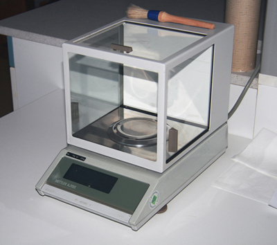
Figure 1.23 Many mechanical balances, such as double-pan balances, have been replaced by digital scales, which can typically measure the mass of an object more
precisely. Whereas a mechanical balance may only read the mass of an object to the nearest tenth of a gram, many digital scales can measure the mass of an object up to the
nearest thousandth of a gram. (credit: Karel Jakubec)
Accuracy and Precision of a Measurement
Science is based on observation and experiment—that is, on measurements. Accuracy is how close a measurement is to the correct value for that
measurement. For example, let us say that you are measuring the length of standard computer paper. The packaging in which you purchased the
paper states that it is 11.0 inches long. You measure the length of the paper three times and obtain the following measurements: 11.1 in., 11.2 in., and
10.9 in. These measurements are quite accurate because they are very close to the correct value of 11.0 inches. In contrast, if you had obtained a
measurement of 12 inches, your measurement would not be very accurate.
The precision of a measurement system is refers to how close the agreement is between repeated measurements (which are repeated under the
same conditions). Consider the example of the paper measurements. The precision of the measurements refers to the spread of the measured
values. One way to analyze the precision of the measurements would be to determine the range, or difference, between the lowest and the highest
measured values. In that case, the lowest value was 10.9 in. and the highest value was 11.2 in. Thus, the measured values deviated from each other
by at most 0.3 in. These measurements were relatively precise because they did not vary too much in value. However, if the measured values had
been 10.9, 11.1, and 11.9, then the measurements would not be very precise because there would be significant variation from one measurement to
another.
The measurements in the paper example are both accurate and precise, but in some cases, measurements are accurate but not precise, or they are
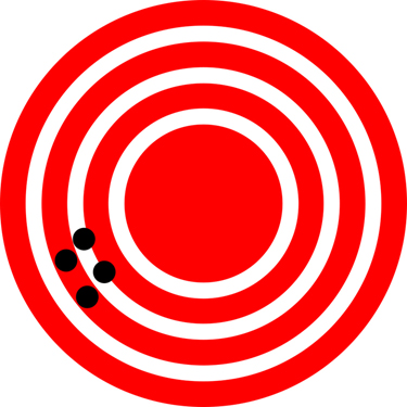
precise but not accurate. Let us consider an example of a GPS system that is attempting to locate the position of a restaurant in a city. Think of the
restaurant location as existing at the center of a bull’s-eye target, and think of each GPS attempt to locate the restaurant as a black dot. In Figure
1.24, you can see that the GPS measurements are spread out far apart from each other, but they are all relatively close to the actual location of the restaurant at the center of the target. This indicates a low precision, high accuracy measuring system. However, in Figure 1.25, the GPS
measurements are concentrated quite closely to one another, but they are far away from the target location. This indicates a high precision, low
accuracy measuring system.
26 CHAPTER 1 | INTRODUCTION: THE NATURE OF SCIENCE AND PHYSICS
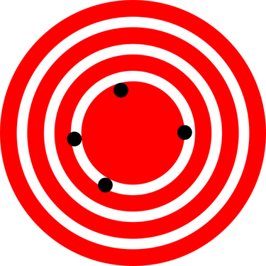
Figure 1.24 A GPS system attempts to locate a restaurant at the center of the bull’s-eye. The black dots represent each attempt to pinpoint the location of the restaurant. The
dots are spread out quite far apart from one another, indicating low precision, but they are each rather close to the actual location of the restaurant, indicating high accuracy.
(credit: Dark Evil)
Figure 1.25 In this figure, the dots are concentrated rather closely to one another, indicating high precision, but they are rather far away from the actual location of the
restaurant, indicating low accuracy. (credit: Dark Evil)
Accuracy, Precision, and Uncertainty
The degree of accuracy and precision of a measuring system are related to the uncertainty in the measurements. Uncertainty is a quantitative
measure of how much your measured values deviate from a standard or expected value. If your measurements are not very accurate or precise, then
the uncertainty of your values will be very high. In more general terms, uncertainty can be thought of as a disclaimer for your measured values. For
example, if someone asked you to provide the mileage on your car, you might say that it is 45,000 miles, plus or minus 500 miles. The plus or minus
amount is the uncertainty in your value. That is, you are indicating that the actual mileage of your car might be as low as 44,500 miles or as high as
45,500 miles, or anywhere in between. All measurements contain some amount of uncertainty. In our example of measuring the length of the paper,
we might say that the length of the paper is 11 in., plus or minus 0.2 in. The uncertainty in a measurement, A , is often denoted as δA (“delta A ”),
so the measurement result would be recorded as A ± δA . In our paper example, the length of the paper could be expressed as 11 in. ± 0.2.
The factors contributing to uncertainty in a measurement include:
1. Limitations of the measuring device,
2. The skill of the person making the measurement,
3. Irregularities in the object being measured,
4. Any other factors that affect the outcome (highly dependent on the situation).
In our example, such factors contributing to the uncertainty could be the following: the smallest division on the ruler is 0.1 in., the person using the
ruler has bad eyesight, or one side of the paper is slightly longer than the other. At any rate, the uncertainty in a measurement must be based on a
careful consideration of all the factors that might contribute and their possible effects.
Making Connections: Real-World Connections – Fevers or Chills?
Uncertainty is a critical piece of information, both in physics and in many other real-world applications. Imagine you are caring for a sick child.
You suspect the child has a fever, so you check his or her temperature with a thermometer. What if the uncertainty of the thermometer were
3.0ºC ? If the child’s temperature reading was 37.0ºC (which is normal body temperature), the “true” temperature could be anywhere from a
hypothermic 34.0ºC to a dangerously high 40.0ºC . A thermometer with an uncertainty of 3.0ºC would be useless.
Percent Uncertainty
One method of expressing uncertainty is as a percent of the measured value. If a measurement A is expressed with uncertainty, δA , the percent
uncertainty (%unc) is defined to be
(1.8)
% unc = δA
A ×100%.
CHAPTER 1 | INTRODUCTION: THE NATURE OF SCIENCE AND PHYSICS 27
Example 1.2 Calculating Percent Uncertainty: A Bag of Apples
A grocery store sells 5-lb bags of apples. You purchase four bags over the course of a month and weigh the apples each time. You obtain the
following measurements:
• Week 1 weight: 4.8 lb
• Week 2 weight: 5.3 lb
• Week 3 weight: 4.9 lb
• Week 4 weight: 5.4 lb
You determine that the weight of the 5-lb bag has an uncertainty of ±0.4 lb . What is the percent uncertainty of the bag’s weight?
Strategy
First, observe that the expected value of the bag’s weight, A , is 5 lb. The uncertainty in this value, δA , is 0.4 lb. We can use the following
equation to determine the percent uncertainty of the weight:
(1.9)
% unc = δA
A ×100%.
Solution
Plug the known values into the equation:
(1.10)
% unc =0.4 lb
5 lb ×100% = 8%.
Discussion
We can conclude that the weight of the apple bag is 5 lb ± 8% . Consider how this percent uncertainty would change if the bag of apples were
half as heavy, but the uncertainty in the weight remained the same. Hint for future calculations: when calculating percent uncertainty, always
remember that you must multiply the fraction by 100%. If you do not do this, you will have a decimal quantity, not a percent value.
Uncertainties in Calculations
There is an uncertainty in anything calculated from measured quantities. For example, the area of a floor calculated from measurements of its length
and width has an uncertainty because the length and width have uncertainties. How big is the uncertainty in something you calculate by multiplication
or division? If the measurements going into the calculation have small uncertainties (a few percent or less), then the method of adding percents can
be used for multiplication or division. This method says that the percent uncertainty in a quantity calculated by multiplication or division is the sum of
the percent uncertainties in the items used to make the calculation. For example, if a floor has a length of 4.00 m and a width of 3.00 m , with
uncertainties of 2% and 1% , respectively, then the area of the floor is 12.0 m2 and has an uncertainty of 3% . (Expressed as an area this is
0.36 m2 , which we round to 0.4 m2 since the area of the floor is given to a tenth of a square meter.)
A high school track coach has just purchased a new stopwatch. The stopwatch manual states that the stopwatch has an uncertainty of ±0.05 s
. Runners on the track coach’s team regularly clock 100-m sprints of 11.49 s to 15.01 s . At the school’s last track meet, the first-place sprinter
came in at 12.04 s and the second-place sprinter came in at 12.07 s . Will the coach’s new stopwatch be helpful in timing the sprint team?
Why or why not?
Solution
No, the uncertainty in the stopwatch is too great to effectively differentiate between the sprint times.
Precision of Measuring Tools and Significant Figures
An important factor in the accuracy and precision of measurements involves the precision of the measuring tool. In general, a precise measuring tool
is one that can measure values in very small increments. For example, a standard ruler can measure length to the nearest millimeter, while a caliper
can measure length to the nearest 0.01 millimeter. The caliper is a more precise measuring tool because it can measure extremely small differences
in length. The more precise the measuring tool, the more precise and accurate the measurements can be.
When we express measured values, we can only list as many digits as we initially measured with our measuring tool. For example, if you use a